The Connectionist Temporal Classification is a type of scoring function for the output of neural networks where the input sequence may not align with the output sequence at every timestep. It was first introduced in the paper by [Alex Graves et al] for labelling unsegmented phoneme sequence. It has been successfully applied in other classification tasks such as speech recognition, keyword spotting, handwriting recognition, video description. These tasks require alignment between the input and output which may not be given. Therefore, it has become an ubiquitous loss for tasks requiring dynamic alignment of input to output. In this article, we will breakdown the inner workings of the CTC loss computation using the forward-backward algorithm.
We will not be discussing the decoding methods used during inference such as beam search with ctc or prefix search. For an introductory look at CTC, you can read Sequence Modeling With CTC by Awni Hannun.
Here’s what we will cover:
Introduction
Let’s look an automatic speech recognition task where we have to predict the words spoken from the audio data.

Looking at the speech segment, how can we align the words to where they are spoken in the speech segment? Even if it is possible to manually do it for this task, it is not feasible for a large corpus of audio data.
With the CTC alignment, we do not require alignment between input and output sequence (in terms of location). CTC tries all possible alignments of the ground truth to the prediction.
The CTC Model
Let’s get concrete with what we have been talking about by designing a task and apply the CTC loss.
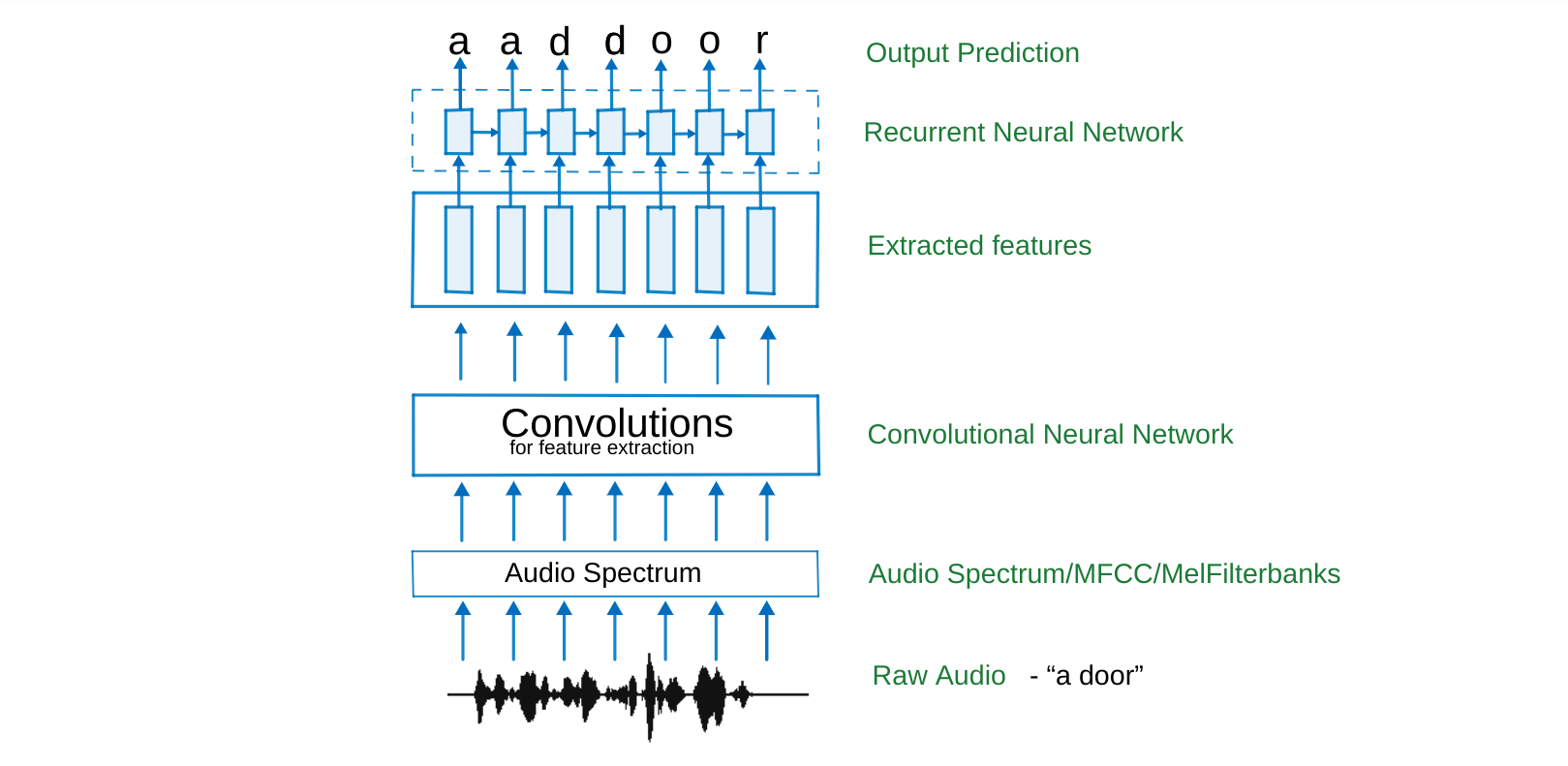
In the model above, we convert the raw audio signal into its spectrum or apply melfiterbanks (this is optional and can be performed by a CNN layer), which is then passed through a convolution neural network (CNN). CNNs enable us extract features, by looking at a window of the data while performing strided convolutions along the feature dimension of the audio.
The features are then passed through a Recurrent Neural Network (RNN) for decoding. At the decoding stage, if we perform a max decoding at each timestep, we will get tokens of a much longer length than the input, which naturally implies that redundant tokens will be decoded to fill up some of the timesteps. How do we contract the decoded output to represent our predictions? How should we deal with silences in the audio? How should we indicate repetitions of tokens as in “d-oo-r”?
Well, Instead of decoding characters, we can decode phonemes, subwords, or even words depending on the task. Let’s consider the instance of character decoding for this article.
We can solve these problems by explicitly introducing a blank token into our vocabulary to cater for these dynamics. We further include a separator token to indicate spaces between each word.
Thus, “a door” split into [“ε”, “a”, “_”, “d”, “o”, “o”, “r”] tokens is then transformed into [“ε”, “a”, “ε”, “_”, “ε”, “d”, “ε”, “o”, “ε”, “o”, “ε”, “r”, “ε”] where the blank token is included. With this, we know that we can only have repeating tokens only if they are separated by a blank token, “ε” e.g. “d”, “o”, “ε”, “o”, “ε”, “r” is allowed and not “d”, “o”, “o”, “ε”, “r”. The latter contracts into “dor”.
In general, given an initial sequence of length $M$, the length of the expanded sequence is $2*M + 1$
Getting into ctc details
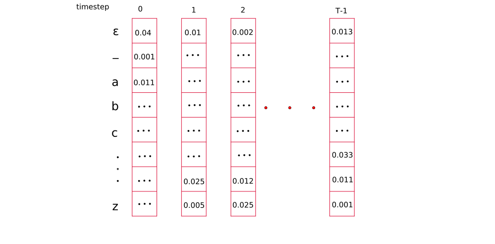
At the output of the RNN, we get a vector, which has the length of vocabulary, for each time step of RNN computation. The softmax function is applied to it to get a vector of probabilities. The number of output labels cannot be more than the number of features from the CNN, so the features has to be estimated accordingly (by taking the maximum length of sequence in vocabulary or some other heuristic).
We will consider a smaller label “door” which should be enough to explain the entire concept succinctly. Let’s generate our vocabulary as the standard lowercase alphabets, including our special tokens.
[“ε”:0, “_“:1, “a”: 2, “b”:3, … ,”z”:28]
We denote the total number of timesteps by $T$, length of the expanded target output by $S$, and length of label by $M$. So, $S = 2*M + 1$ e.g for “door”, $S = 2*4+1$
Given these vectors of probability distributions, how do we learn the alignments of the probable predictions? We need a structured way to traverse from the first softmax distribution to the last to represent the word.
Setting up constrains on the alignment
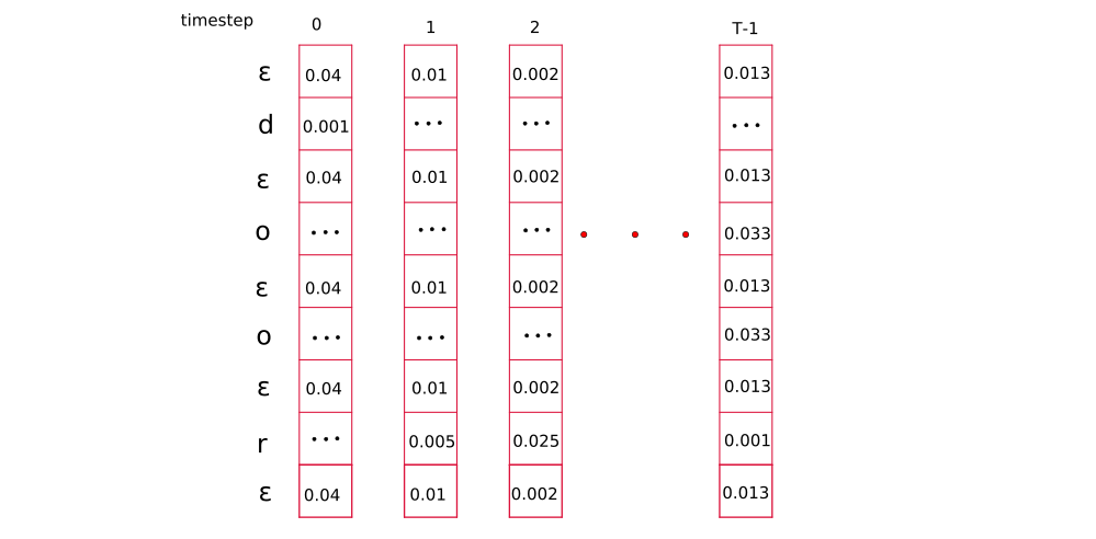
In principle, we exclude all rows that do not include tokens from the target sequence and then rearrange the tokens to form the output sequence. This is done during training only. At inference, a beam search can be performed on the distribution. So, we copy the required output for the target into a secondary reduced structure and decode on the reduced structure assuring us that only appropriate tokens will be used for selected for computing loss and gradients.
If a token occur multiple times in the label, we repeat the rows for similar tokens in their appropriate location. This becomes our probability matrix, $y_{(s, t)}$
Composing the graph
Now that we have our full grid, we can begin traversing the grid from top-left to bottom right in such a way that; (a) the first character in the decoding must be a blank token, ‘ε’ or the first sequence token ‘d’ (b) the last token is either a blank token or the last sequence token ‘r’ (c) the rest of the sequence follows a sequence path that monotonically travels down from the top-left to bottom-right.
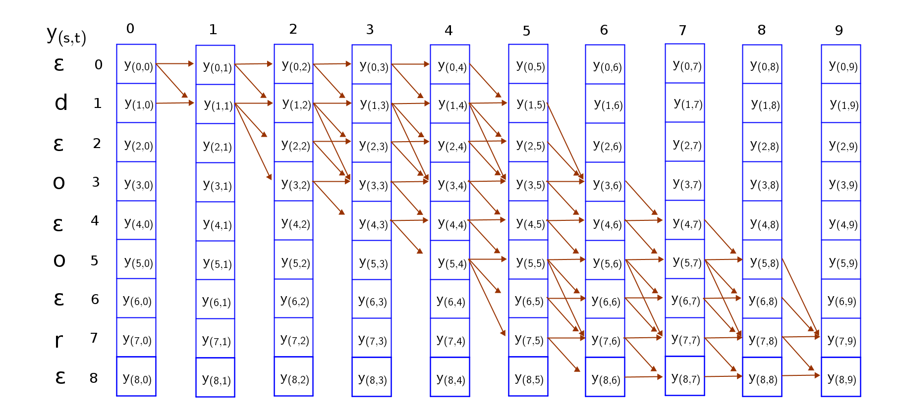
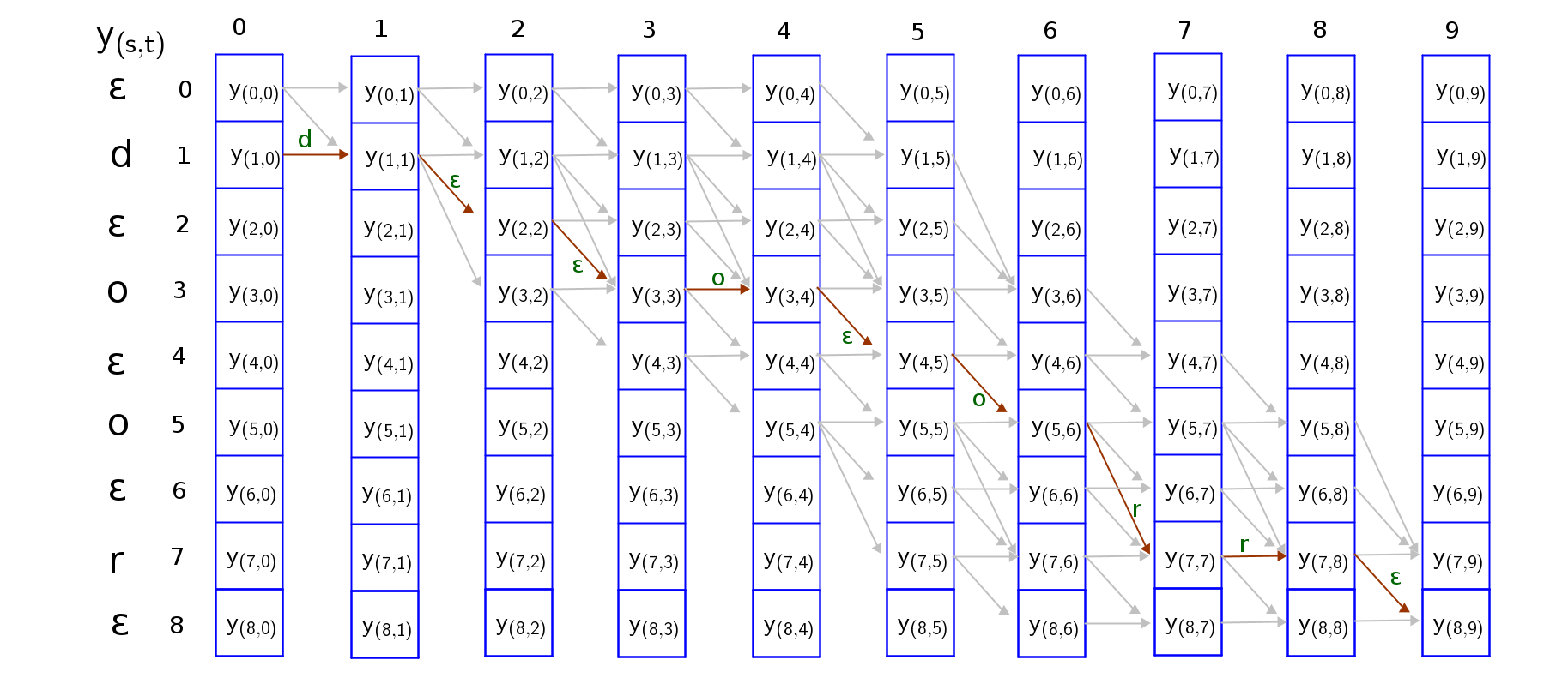
To guarantee that the sequence is an expansion of the target sequence, we can only traverse the grid through these valid paths from top-left to bottom-right. I have attempted to trave all paths in the grid, and you can do it as an exercise too. Two valid paths where both collapse into “door” are shown below;
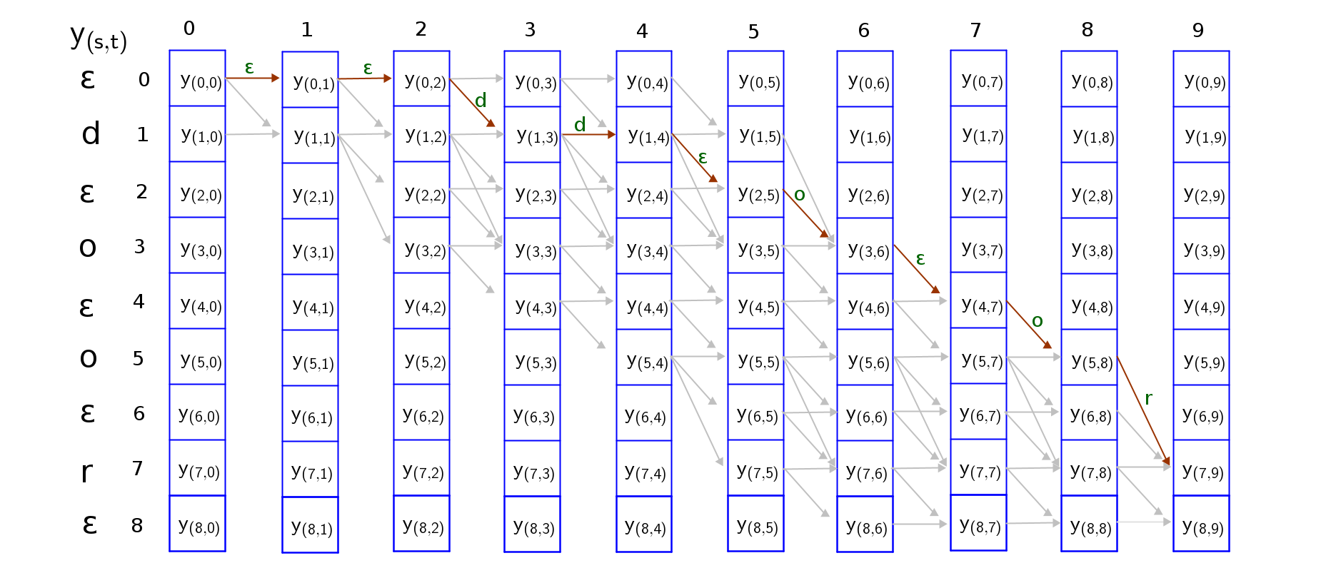
It is easy to trace these paths if we consider the following traversal rules;
- The sequence can start with a blank token or the first character token and end with a blank token or the last character token. So we have to consider both paths.
- Skips are permitted across a blank token only if the tokens on either side of the blank token are different because a blank is required to distinguish repetition of a token but not required between distinct tokens
Scoring the paths
The score of a path is the product of probabilities of all nodes along the path. For the two paths considered in the examples above.
$score(pathA) = y_{(0,0)}*y_{(0,1)}*y_{(0,2)}*y_{(1,3)}*y_{(1,4)}*y_{(2,5)}*y_{(3,6)}*y_{(4,7)}*y_{(5,8)}*y_{(7,9)}$
$score(pathB) = y_{(1,0)}*y_{(1,1)}*y_{(2,2)}*y_{(3,3)}*y_{(3,4)}*y_{(4,5)}*y_{(5,6)}*y_{(7,7)}*y_{(7,8)}*y_{(8,9)}$
We are required to trace out all the possible paths that contract into “door” and there are an exponential number of such valid paths as can be seen from the graph. The complexity is of the order $\mathcal{O}(|V|^T)$ where $|V|$ is the length of vocabulary.
Can we find a dynamic programming algorithm for solving this problem? Well, the viterbi algorithm can generate the most likely path, and does not guarantee we get the most likely sequence of labels. It finds the best path to a node by extending the best path to one of its parent nodes. Any other path would necessarily have a lower probability. But, the viterbi algorithm commits to a path or initial alignment early (without exploration) which can lead to suboptimal results.
Forward-Backward Algorithm
Instead of only selecting the most likely alignment, we find the expectation over all possible alignments during training. This allows us to also exploit the existence of subpaths in the graph.
To compute this effectively, we need a forward variable $\alpha_{(s, t)}$ and backward variable $\beta_{(s, t)}$ where $s$ is the index of the token considered. The forward variable computes the total probability of a sequence $seq[1:s]$ up to a particular timestep $t$. The backward variable calculates the total probability of remaining sequence from token $seq(s)$ to token $seq(S)$, $seq[s:S]$ at timestep $t$.
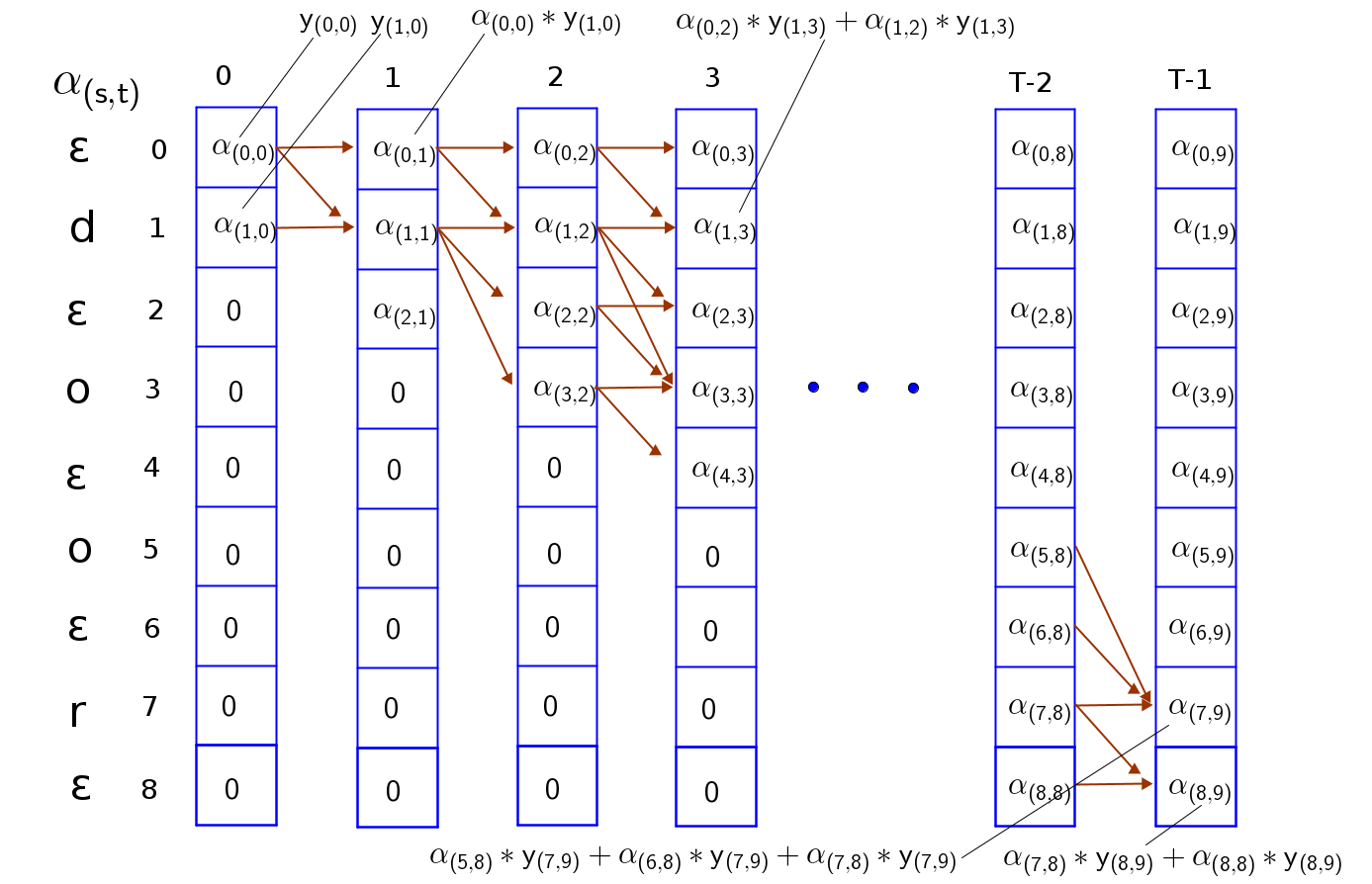
Forward Algorithm for computing $\alpha_{(s, t)}$
First, let’s create a matrix of zeros of same shape as our probability matrix, $y_{(s, t)}$ to store our $\alpha$ values. The forward algorithm is given by;
Initialize:
$\alpha$-mat = zeros_like(y-mat)
$\alpha_{(0, 0)} = y_{(0, 0)}$, $\alpha_{(1, 0)} = y_{(1, 0)}$
$\alpha_{(s, 0)} = 0$ for $s > 1$
Iterate forward:
- for t = 1 to T-1:
- for s = 0 to S:
- $\alpha_{(s, t)} = (\alpha_{(s, t-1)} + \alpha_{(s-1, t-1)})y_{(s, t)}$ if $seq(s) = “ε”$ or seq(s) = seq(s-2)
- $\alpha_{(s, t)} = (\alpha_{(s, t-1)} + \alpha_{(s-1, t-1)} + \alpha_{(s-2, t-2)})y_{(s, t)}$ otherwise
- for s = 0 to S:
Note that $\alpha_{(s, t)} = 0$ for all $s < S-2(T-t) - 1$ which corresponds to the unconnected boxes in the top-right. These variables correspond to states for which there are not enough time-steps left to complete the sequence.
$seq(s)$ - token at index $s$ e.g. $seq(s=1)=”d”$
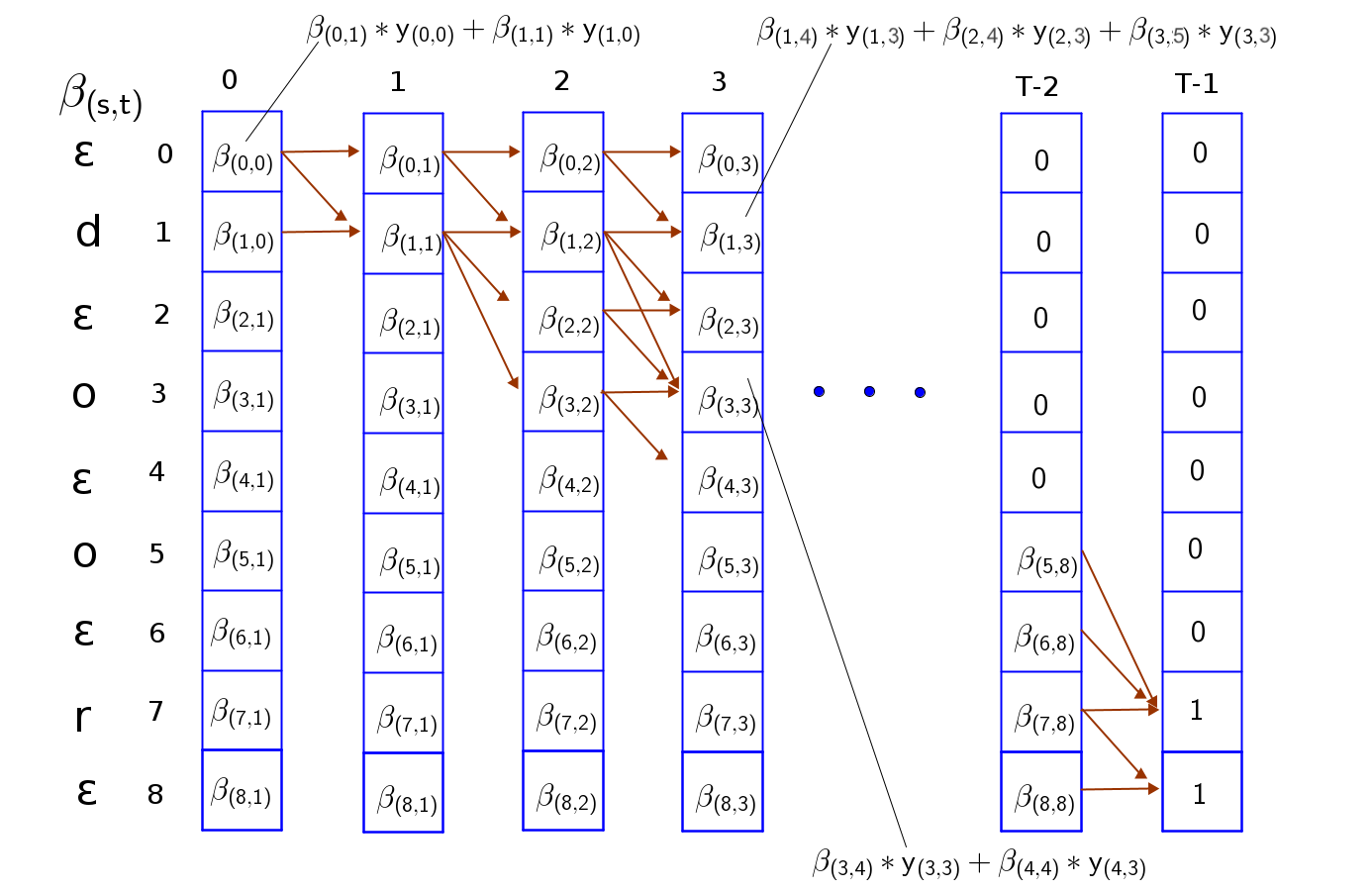
Backward algorithm for computing $\beta_{(s, t)}$
Let’s also create a matrix of zeros of same shape as our probability matrix, $y_{(s, t)}$ to store our $\beta$ values.
Initialize:
- $\beta_{(S-1, T-1)} = 1$, $\beta_{(S-2, T-1)} = 1$,
- $\beta_{(s, T-1)} = 0$ for $s < S-2$
Iterate backward:
- for t = T-2 to 0:
- for s = S-1 to 0:
- $\beta_{(s, t)} = \beta_{(s, t+1)}y_{(s, t)} + \beta_{(s+1, t+1)}y_{(s+1, t)}$ if $seq(s) = “ε”$ or $seq(s) = seq(s+2)$
- $\beta_{(s, t)} = \beta_{(s, t+1)}y_{(s, t)} + \beta_{(s+1, t+1)}y_{(s+1, t)} + \beta_{(s+2, t+2)})y_{(s+2, t)}$ otherwise
- for s = S-1 to 0:
Similarly, $\beta_{(s, t)} = 0$ for all $s > 2t$ which corresponds to the unconnected boxes in the bottom-left.
Computing the probabilities efficiently
From the computations, observe that we are constantly multiplying values less than 1. This can lead to underflow especially for longer sequences. We can improve these computations by performing the computations in the logarithm space. Products become sums, divisions become subtraction. For instance;
$\alpha_{s, t} = (\alpha_{s, t-1} + \alpha_{(s-1, t-1)})y_{s, t}$
becomes
$log \alpha_{s,t} = log( e^{log\alpha_{s,t-1}} + e^{log\alpha_{s-1,t-1}}) + log P_{s,t} $
CTC Loss calculation for each timestep
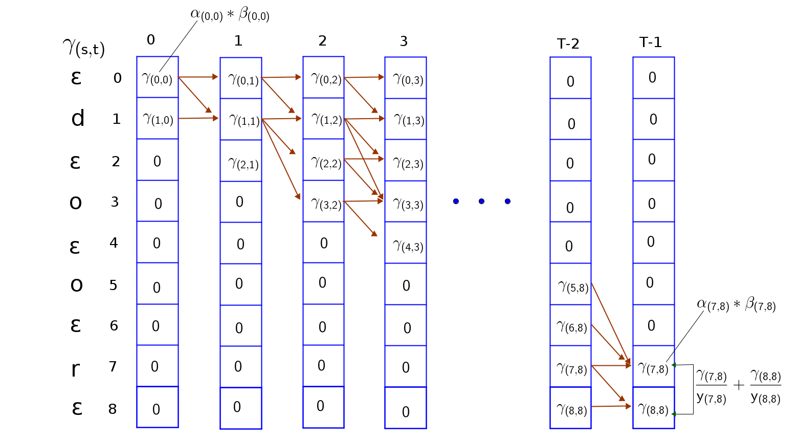
Now that we have the $\alpha$ and $\beta$ probabilities(or log probabilities), we will compute the joint probability of the sequence at every timestep. This we will call $\gamma_{s,t}$.
$\gamma_{s,t} = \alpha_{s,t}\beta_{s,t}$
Afterwards, we compute the posterior probabilities of the sequence at every timestep by summing along columns. This is the total probability of all paths going through a token $seq(s)$ at timestep t.
$P_{(seq_t, t)} = \sum\limits_{s=0}^{S}\dfrac{\alpha_{s,t}\beta_{s,t}}{y_{s,t}}$
Total loss of the model is then;
$\mathcal{l} = -\sum\limits_{t=0}^{T-1} log P_{(seq_t, t)}$
Derivatives can then be calculated for back propagation using Autograd. Modern deep leaning libraries such as Pytorch, and TensorFlow have this feature.
Note
- The CTC loss algorithm can be applied to both convolutional and recurrent networks. For recurrent networks, it is possible to compute the loss at each timestep in the path or make use of the final loss, depending on the use case.
- Some forms of the loss use only the forward algorithm in its computation i.e $\alpha_{s, t}$. I was only able to reproduce the Pytorch CTC loss when I used the forward algorithm in my loss computation, and ignoring the backward algorithm. However, the algorithm explained in this blog post is the one proposed in the seminal paper by [Alex Graves et al].
Conclusion
In this article, we explained the connectionist temporal classification loss and how it can be applied in many-to-many input/output classification tasks without alignments. Then, we showed the computations for the forward and backward algorithm used for the training the model.
References
- Hannun, “Sequence Modeling with CTC”, Distill, 2017.
- Bhiksha Raj, Connectionist Temporal Classification (CTC) lecture slide, link, last retrieved July 2020.