<?xml version="1.0" encoding="utf-8"?><feed xmlns="http://www.w3.org/2005/Atom" xml:lang="en"><generator uri="https://jekyllrb.com/" version="3.10.0">Jekyll</generator><link href="https://ogunlao.github.io/feed.xml" rel="self" type="application/atom+xml" /><link href="https://ogunlao.github.io/" rel="alternate" type="text/html" hreflang="en" /><updated>2026-10-07T23:50:37+00:00</updated><id>https://ogunlao.github.io/feed.xml</id><title type="html">Sewade Ogun</title><subtitle>Sewade Ogun&apos;s blog. Notes on the rapidly changing field of AI, mostly through the lens of multimodality: speech language models, TTS, ASR and LLMs.</subtitle><author><name>Sewade Ogun</name><email>sogun@aimsammi.org</email></author><entry><title type="html">Consider using UAR instead of Accuracy for Imbalanced Classification tasks</title><link href="https://ogunlao.github.io/blog/2021/04/24/consider_uar_accuracy.html" rel="alternate" type="text/html" title="Consider using UAR instead of Accuracy for Imbalanced Classification tasks" /><published>2021-04-24T00:00:00+00:00</published><updated>2021-04-24T00:00:00+00:00</updated><id>https://ogunlao.github.io/blog/2021/04/24/consider_uar_accuracy</id><content type="html" xml:base="https://ogunlao.github.io/blog/2021/04/24/consider_uar_accuracy.html"><![CDATA[<p>Accuracy is one  of the most used metrics to evaluate classification tasks in machine learning. It is the ratio of the number of correct predictions to the total number of examples. It is simple to understand and compute, which makes it an easy evaluation metric to optimize but it has its shortcomings. Many other metrics such as precision, recall, F1-score etc have majorly been used to sidestep its limitations, but I will like to argue for the Unweighted Average Recall as a good or even better metric to optimize when the sample class ratio is imbalanced, and it is closely related to the accuracy.</p>

<p>Here’s what we will cover:</p>
<ol id="markdown-toc">
  <li><a href="#introduction" id="markdown-toc-introduction">Introduction</a></li>
  <li><a href="#decomposing-the-accuracy-score" id="markdown-toc-decomposing-the-accuracy-score">Decomposing the accuracy score</a></li>
  <li><a href="#balanced-classification-accuracy-or-unweighted-average-recall" id="markdown-toc-balanced-classification-accuracy-or-unweighted-average-recall">Balanced Classification Accuracy or Unweighted Average Recall</a></li>
  <li><a href="#how-this-is-computed" id="markdown-toc-how-this-is-computed">How this is computed</a></li>
  <li><a href="#conclusion" id="markdown-toc-conclusion">Conclusion</a></li>
</ol>

<h2 id="introduction">Introduction</h2>

<p>Given a set of samples \(\mathcal{X}\) with corresponding labels \(\mathcal{Y}\). Let us assume we have a binary classification task with only two labels, \(y_1\) and \(y_2\).</p>

<p>We can train a classifier using binary cross-entropy loss, hinge loss (or whatever loss is fit) to get the best model for our task. Afterwards, we evaluate this model on unseen data to determine how well it generalizes. This is commonly done by calculating a score like accuracy.</p>

<h2 id="decomposing-the-accuracy-score">Decomposing the accuracy score</h2>

<p>Accuracy can be computed from the confusion matrix, which gives a breakdown of prediction scores such as true positive \((tp)\), true negative \((tn)\), false positive \((fp)\) and false negative \((fn)\). The goal of this article is not to explain these terms, since there are other great articles online on the subject of confusion matrix.</p>

\[\text{accuracy} = \dfrac{\text{total correct predictions}}{\text{total number of predictions}}\]

<p>This can be shown to correspond the following from the confusion matrix;</p>

\[\begin{aligned}
\text{accuracy} &amp;= \dfrac{tp + tn}{tp + tn + fp + fn} \\
     &amp;= \dfrac{tp + tn}{p + n}
\end{aligned}\]

<p>where \(p\) is the total no. of positives and \(n\) is the total no. of negatives.</p>

<p>The class label we use as positive or negative is arbitrary here. We can further decompose the equation above into two parts;</p>

\[\text{accuracy} = \dfrac{tp}{p + n} + \dfrac{tn}{p + n}\]

<p>Multiplying the first part by \(p\) and second part by \(n\) clearly becomes;</p>

\[\text{accuracy} = \dfrac{tp}{p} \cdot \dfrac{p}{p + n} + \dfrac{tn}{n} \cdot \dfrac{n}{p + n}\]

<p>Let’s take the individual elements of the last equation to motivate the UAR.</p>

<ul>
  <li>\(\dfrac{tp}{p}\) is known as the Recall on the positive class and it is the ratio of the total correctly predicted positives to the total number of positives. It is also known as Sensitivity</li>
  <li>\(\dfrac{tn}{n}\) is known as the Recall on the negative class and it is the ratio of the total correctly predicted negative to the total number of negatives. It is also known as Specificity</li>
</ul>

<p>The accuracy score can then be written as follows;</p>

\[\text{accuracy} = \text{Sensitivity} \cdot \dfrac{p}{p + n} + \text{Specificity} \cdot \dfrac{n}{p + n}\]

<p>\(\dfrac{p}{p + n}\) and \(\dfrac{n}{p + n}\) are weights applied to the sensitivity and specificity and both sum to 1. These weights apply a higher score to the recall with more class samples and lower to the other, so it does not weigh the two classes equally. This makes it generally unfit for understanding how well the model is performing for very skewed datasets.</p>

<h2 id="balanced-classification-accuracy-or-unweighted-average-recall">Balanced Classification Accuracy or Unweighted Average Recall</h2>

<p>To mitigate the bias in weighting, we can simply replace the weights with 0.5 or \(\dfrac{1}{\text{no. of classes}}\) for the multiclass scenario.</p>

<p>The balanced accuracy then becomes;</p>

\[\text{accuracy}_{\text{bal}} = \text{Sensitivity} \times 0.5 + \text{Specificity} \times 0.5\]

<p>This balanced accuracy is known as the Unweighted Average Recall, the average of the recall on the positive class and recall on the negative class. There is a correlation between the accuracy and UAR but the UAR gives the correct expectation on class predictions.</p>

<h2 id="how-this-is-computed">How this is computed</h2>

<p>This can be computed from a confusion matrix. Below is a function that computes specificity, sensitivity, accuracy and uar in python given the confusion matrix.</p>

<div class="language-python highlighter-rouge"><div class="highlight"><pre class="highlight"><code><span class="k">def</span> <span class="nf">compute_metrics</span><span class="p">(</span><span class="n">confusion_matrix</span><span class="p">):</span>
    <span class="s">"""Calculates specificity, sensitivity, accuracy and uar from confusion matrix
    Confusion matrix of form [[tp, fp]
                              [fn, tn]]
    args:
      confusion_matrix: 2 by 2 nd-array
      output: tuple of float (specificity, sensitivity, accuracy, uar)
    """</span>
    <span class="n">cm</span> <span class="o">=</span> <span class="n">confusion_matrix</span>
    <span class="n">tp</span><span class="p">,</span> <span class="n">tn</span> <span class="o">=</span> <span class="n">cm</span><span class="p">[</span><span class="mi">0</span><span class="p">,</span> <span class="mi">0</span><span class="p">],</span> <span class="n">cm</span><span class="p">[</span><span class="mi">1</span><span class="p">,</span> <span class="mi">1</span><span class="p">]</span>
    <span class="n">fn</span><span class="p">,</span> <span class="n">fp</span> <span class="o">=</span> <span class="n">cm</span><span class="p">[</span><span class="mi">1</span><span class="p">,</span> <span class="mi">0</span><span class="p">],</span> <span class="n">cm</span><span class="p">[</span><span class="mi">0</span><span class="p">,</span> <span class="mi">1</span><span class="p">]</span>
    
    <span class="n">sensitivity</span> <span class="o">=</span> <span class="n">tp</span> <span class="o">/</span> <span class="p">(</span><span class="n">tp</span> <span class="o">+</span> <span class="n">fn</span><span class="p">)</span>
    <span class="n">specificity</span> <span class="o">=</span> <span class="n">tn</span> <span class="o">/</span> <span class="p">(</span><span class="n">fp</span> <span class="o">+</span> <span class="n">tn</span><span class="p">)</span>
    
    <span class="n">uar</span> <span class="o">=</span> <span class="p">(</span><span class="n">specificity</span> <span class="o">+</span> <span class="n">sensitivity</span><span class="p">)</span><span class="o">/</span><span class="mf">2.0</span>
    
    <span class="n">accuracy</span> <span class="o">=</span> <span class="p">(</span><span class="n">tp</span> <span class="o">+</span> <span class="n">tn</span><span class="p">)</span> <span class="o">/</span> <span class="p">(</span><span class="n">tp</span> <span class="o">+</span> <span class="n">tn</span> <span class="o">+</span> <span class="n">fp</span> <span class="o">+</span> <span class="n">fn</span><span class="p">)</span>
    
    <span class="n">metrics_dict</span> <span class="o">=</span> <span class="nb">dict</span><span class="p">(</span><span class="n">sensitivity</span><span class="o">=</span><span class="n">sensitivity</span><span class="p">,</span> <span class="n">specificity</span><span class="o">=</span><span class="n">specificity</span><span class="p">,</span> 
                       <span class="n">accuracy</span><span class="o">=</span><span class="n">accuracy</span><span class="p">,</span> <span class="n">uar</span><span class="o">=</span><span class="n">uar</span><span class="p">)</span>
    <span class="k">return</span> <span class="n">metrics_dict</span>
</code></pre></div></div>

<p>Let us look at some cases of how accuracy and UAR differ in their metrics</p>

<p><strong>Case 1: Balanced class</strong>
Here, we have 50 samples from the positive class and 50 samples from the negative class. The model predicts 45 of 50 samples correctly for the positive class and 39 of 50 samples correctly for the negative class.</p>

<div class="language-python highlighter-rouge"><div class="highlight"><pre class="highlight"><code><span class="o">&gt;&gt;</span> <span class="kn">import</span> <span class="nn">numpy</span> <span class="k">as</span> <span class="n">np</span>
<span class="o">&gt;&gt;</span> <span class="n">cm</span> <span class="o">=</span> <span class="n">np</span><span class="p">.</span><span class="n">array</span><span class="p">([[</span><span class="mi">45</span><span class="p">,</span> <span class="mi">11</span><span class="p">],</span>
                  <span class="p">[</span><span class="mi">5</span><span class="p">,</span> <span class="mi">39</span><span class="p">]])</span>
<span class="o">&gt;&gt;</span> <span class="k">print</span><span class="p">(</span><span class="n">compute_metrics</span><span class="p">(</span><span class="n">cm</span><span class="p">))</span>
</code></pre></div></div>

<div class="language-python highlighter-rouge"><div class="highlight"><pre class="highlight"><code><span class="c1"># Note that values have been rounded up to 2 decimal places
</span><span class="n">output</span><span class="p">:</span> <span class="p">{</span><span class="s">'sensitivity'</span><span class="p">:</span> <span class="mf">0.90</span><span class="p">,</span> <span class="s">'specificity'</span><span class="p">:</span> <span class="mf">0.78</span><span class="p">,</span> <span class="s">'accuracy'</span><span class="p">:</span> <span class="mf">0.84</span><span class="p">,</span> <span class="s">'uar'</span><span class="p">:</span> <span class="mf">0.84</span><span class="p">}</span>
</code></pre></div></div>

<p>Since the classes are balanced, the UAR and accuracy both give similar information</p>

<p><strong>Case 2: Imbalanced class</strong>
In this case, we have 20 samples from the positive class and 80 samples from negative class. The model predicts 4 of 20 samples correctly for the positive class and 75 of 80 samples correcly for the negative class.</p>

<div class="language-python highlighter-rouge"><div class="highlight"><pre class="highlight"><code><span class="o">&gt;&gt;</span> <span class="n">cm</span> <span class="o">=</span> <span class="n">np</span><span class="p">.</span><span class="n">array</span><span class="p">([[</span><span class="mi">4</span><span class="p">,</span> <span class="mi">5</span><span class="p">],</span>
                  <span class="p">[</span><span class="mi">16</span><span class="p">,</span> <span class="mi">75</span><span class="p">]])</span>
<span class="o">&gt;&gt;</span> <span class="k">print</span><span class="p">(</span><span class="n">compute_metrics</span><span class="p">(</span><span class="n">cm</span><span class="p">))</span>
</code></pre></div></div>

<div class="language-python highlighter-rouge"><div class="highlight"><pre class="highlight"><code><span class="n">output</span><span class="p">:</span> <span class="p">{</span><span class="s">'sensitivity'</span><span class="p">:</span> <span class="mf">0.20</span><span class="p">,</span> <span class="s">'specificity'</span><span class="p">:</span> <span class="mf">0.94</span><span class="p">,</span> <span class="s">'accuracy'</span><span class="p">:</span> <span class="mf">0.79</span><span class="p">,</span> <span class="s">'uar'</span><span class="p">:</span> <span class="mf">0.57</span><span class="p">}</span>
</code></pre></div></div>

<p>Here, the accuracy is over optimistic and indicating that we are doing well on about \(79 \%\) of the samples. This is because of the size of samples of the negative class. However, the UAR gives a truer result showing that we still have work to do. Looking at the specificity and sensitivity closely, they show where the problem lies. The model is doing poorly on the positive class (as indicated by the sensitivity, \(20 \%\))</p>

<p>You can play with different formulations of the confusion matrix to better understand how class imbalance affects the scores.</p>

<blockquote>
  <p>I first saw the UAR score on <a href="https://onucharles.github.io/">Charles Onu</a>’s Master thesis in the section “Balanced Classification Accuracy and Misclassification Loss”. This is a decomposition of the equation.</p>
</blockquote>

<p><strong>Update</strong>
Sep 11, 21: Fixed in a bug in computing the UAR in an earlier version of this article, and added clearer examples</p>

<h2 id="conclusion">Conclusion</h2>

<p>Accuracy is the most used metric for evaluating machine learning classification tasks. In this article, we decomposed the accuracy into individual ratios composed of the sensitivity and specificity weighted by a class ratio. Then, we fixed the bias in the accuracy by giving equal weights to both scores. This led to the Unweighted Average Recall.</p>]]></content><author><name>Sewade Ogun</name><email>sogun@aimsammi.org</email></author><category term="blog" /><category term="metrics" /><summary type="html"><![CDATA[Accuracy is one of the most used metrics to evaluate classification tasks in machine learning. It is the ratio of the number of correct predictions to the total number of examples. It is simple to understand and compute, which makes it an easy evaluation metric to optimize but it has its shortcomings. Many other metrics such as precision, recall, F1-score etc have majorly been used to sidestep its limitations, but I will like to argue for the Unweighted Average Recall as a good or even better metric to optimize when the sample class ratio is imbalanced, and it is closely related to the accuracy.]]></summary></entry><entry><title type="html">How to create a speech dataset for ASR, TTS, and other speech tasks</title><link href="https://ogunlao.github.io/blog/2021/01/26/how-to-create-speech-dataset.html" rel="alternate" type="text/html" title="How to create a speech dataset for ASR, TTS, and other speech tasks" /><published>2021-01-26T00:00:00+00:00</published><updated>2021-01-26T00:00:00+00:00</updated><id>https://ogunlao.github.io/blog/2021/01/26/how-to-create-speech-dataset</id><content type="html" xml:base="https://ogunlao.github.io/blog/2021/01/26/how-to-create-speech-dataset.html"><![CDATA[<p>Over the past few months, I have come across a plethora of questions related to dataset creation for speech projects. I could not find a concise resource detailing all the necessary factors that need to be put in place to have a well balanced, unbiased and clean speech corpus. Many of the answers are distributed across research papers, online platforms and data repositories. As it is well known in the Machine Learning community, creating good datasets for predictive tasks require a ton of effort and attention to detail to get the right results. This article will report my findings on dataset creation for speech related tasks. It will be most useful for students, software engineers and researchers preparing to create their own corpus for specific tasks, especially in the low resource domain. The focus will be on creating corpus for Automatic Speech Recognition (ASR) but the ideas will still be useful for Text-To-Speech(TTS), Speech translation, Speaker classification and other machine learning tasks requiring speech as a modality.</p>

<p>Here’s what we’ll cover:</p>
<ol id="markdown-toc">
  <li><a href="#introduction" id="markdown-toc-introduction">Introduction</a></li>
  <li><a href="#getting-started" id="markdown-toc-getting-started">Getting Started</a>    <ol>
      <li><a href="#sampling-frequency" id="markdown-toc-sampling-frequency">Sampling Frequency</a></li>
      <li><a href="#audio-format-and-encoding" id="markdown-toc-audio-format-and-encoding">Audio Format and Encoding</a></li>
      <li><a href="#length-of-recordings" id="markdown-toc-length-of-recordings">Length of Recordings</a></li>
      <li><a href="#labels" id="markdown-toc-labels">Labels</a></li>
      <li><a href="#number-of-speakers" id="markdown-toc-number-of-speakers">Number of Speakers</a></li>
    </ol>
  </li>
  <li><a href="#annotator-characteristics" id="markdown-toc-annotator-characteristics">Annotator Characteristics</a>    <ol>
      <li><a href="#gender" id="markdown-toc-gender">Gender</a></li>
      <li><a href="#age-groups" id="markdown-toc-age-groups">Age Groups</a></li>
      <li><a href="#accents" id="markdown-toc-accents">Accents</a></li>
      <li><a href="#other-metadata" id="markdown-toc-other-metadata">Other Metadata</a></li>
    </ol>
  </li>
  <li><a href="#other-important-details-to-note" id="markdown-toc-other-important-details-to-note">Other important details to note</a>    <ol>
      <li><a href="#size-of-the-data" id="markdown-toc-size-of-the-data">Size of the data</a></li>
      <li><a href="#noise-and-artefacts" id="markdown-toc-noise-and-artefacts">Noise and Artefacts</a></li>
      <li><a href="#unlabelled-audio" id="markdown-toc-unlabelled-audio">Unlabelled audio</a></li>
      <li><a href="#data-split" id="markdown-toc-data-split">Data Split</a></li>
      <li><a href="#text-preprocessing" id="markdown-toc-text-preprocessing">Text Preprocessing</a></li>
      <li><a href="#data-augmentation" id="markdown-toc-data-augmentation">Data Augmentation</a></li>
    </ol>
  </li>
  <li><a href="#recording-details" id="markdown-toc-recording-details">Recording details</a>    <ol>
      <li><a href="#recording-tools" id="markdown-toc-recording-tools">Recording tools</a></li>
      <li><a href="#source-of-text" id="markdown-toc-source-of-text">Source of Text</a></li>
    </ol>
  </li>
  <li><a href="#conclusion" id="markdown-toc-conclusion">Conclusion</a></li>
</ol>

<h2 id="introduction">Introduction</h2>

<p>A speech corpus is a database containing audio recordings and the corresponding label. The label depends on the task. For ASR tasks, the label is the text, for TTS, the label is the audio itself, while the input is text. For speaker classification, the label will be the speaker id. Therefore, the label and data depends on the particular task. For ASR, the audio samples and text require that they correspond to the same entity. There is a large amount of recorded audio which can be sourced from podcasts, streaming platforms like Youtube, and even talk shows (if permission is granted to you to use them). While the data is available, there are major problems that should be considered when using them for speech tasks. These include;</p>

<ul>
  <li>they may contain artefacts/noise which are not important to the task and machine learning models may find it hard separating those artefacts from the actual signal,</li>
  <li>recordings may/may not have corresponding transcription which may be needed,</li>
  <li>multiple speakers talking simultaneously in the recordings,</li>
  <li>audio recordings may have to be split into short durations, with alignment performed with the corresponding text,</li>
  <li>Podcasts may have music playing at the background, multiple simultaneous speakers etc.</li>
</ul>

<p>With these problems in mind, you may need to determine if the audio is well suited for your task. In this article, we will focus on read speech for creating our own corpus, instead of relying on pre-recorded audio as explained above.</p>

<p><img src="/images/kate-oseen-XQKUIPjPl-s-unsplash.jpg" alt="Photo by Kate Oseen on Unsplash" /></p>

<h2 id="getting-started">Getting Started</h2>

<p>Since 2015, we have seen advances in using deep neural networks for ASR tasks <a href="https://paperswithcode.com/sota/speech-recognition-on-librispeech-test-clean">[Papers with code]</a>, surpassing previous works using Hidden Markov Models (HMM) with Gaussian Mixtures (GMM) or their ensembles on various speech related task. Also, the introduction of the Connectionist Temporal Classification <a href="https://dl.acm.org/doi/10.1145/1143844.1143891">[A Graves, 2006]</a> Loss to alignment has given a major boost to machine learning tasks like speech where alignment between the audio and text is cumbersome. Using the CTC Loss enables the model to maximize the objective over all possible and correct alignments between the audio and text. With these advancements, creating speech data has become significantly easier than previously imagined, with corpus requiring no alignment between the text and the read speech.</p>

<p>For a detailed introduction to CTC Loss, checkout my blog post on <a href="https://ogunlao.github.io/blog/2020/07/17/breaking-down-ctc-loss.html">[Breaking Down the CTC Loss]</a></p>

<h3 id="sampling-frequency">Sampling Frequency</h3>

<p>44.1kHz is the most common sampling frequency used to produce most digital audio. This ensures that the audio can be reconstructed for frequency below 22.05kHz, since it covers all frequencies that can be heard by a human. ASR experiments do not require that high sampling rate; more common frequencies are 8kHz and 16kHz, with sampling frequency of 16kHz becoming the de facto for speech recognition both in production and research, as there is no significant improvement in using a sampling frequency higher than that, although a lower sampling frequency may reduce accuracy Also, increasing the sampling frequency beyond that just increases the overhead during preprocessing and training, with some training procedures taking twice as much time, without any improvements.</p>

<p>On the converse, modern production quality TTS often use 22.05kHz, 32kHz, 44.1kHz, or 48 kHz sampling rate, as 16kHz is too low to achieve high quality TTS <a href="https://arxiv.org/pdf/1904.02882.pdf">[LibriTTS - Heiga Zen et al.]</a> though many research works still use 16kHz. For TTS, the acoustic model needs to learn the fine-grained acoustic characteristic of the audio to be able to reproduce the same form of signal from text.</p>

<p>During the signal preprocessing, the audio can be downsampled to its required sampling rate.</p>

<h3 id="audio-format-and-encoding">Audio Format and Encoding</h3>

<p>Audio format and encoding are two different things. Most popular file format used for speech-to-text experiments is the “.WAV” format. Since ‘wav’ is just a file format, it will have to be encoded during recording using one of the different encoding formats available such as Linear PCM Encoding.You do not need to worry about the details since this would be taken care of for you during your setup. Encodings can be lossy or lossless, taking up different file sizes and quality.</p>

<p>If your read speech corpus is saved in the MP3 file format, you may have to convert them to “.wav” during the preprocessing stage.</p>

<p>For a brief overview of encodings and audio formats, checkout the article <a href="https://cloud.google.com/speech-to-text/docs/encoding">[Introduction to audio encoding - GCP ]</a></p>

<h3 id="length-of-recordings">Length of Recordings</h3>

<p>For ASR tasks, the length of the audio samples should be smaller than about 30 seconds. Typically, for the ASR tasks I have worked on, the average length of the recordings range between 10 seconds and 15 seconds. The shorter the duration the better for the model, especially for models that use recurrent networks (RNN) for decoding. There is also the problem of long-range temporal dependency that needs to be addressed with long duration. It is also advisable to ensure the variance between the audio duration is small likewise.</p>

<p>In the case of TTS, recordings should be splitted on sentence stops instead of silence intervals, to learn long-term characteristics of speech such as the sentence-level prosody for given a text <a href="https://arxiv.org/pdf/1904.02882.pdf">[LibriTTS - Heiga Zen et al.]</a></p>

<p>Other speech classification tasks such as gender identification and speaker identification don’t require long duration of samples. Typical duration of audio is 2  to 4 secs, which is enough to learn the signal characteristic for each class.</p>

<h3 id="labels">Labels</h3>

<p>As previously mentioned, the task determines the label for the audio. For example, Automatic Speech Translation (AST) requires text in the target language which may differ from the source language/language of the audio.</p>

<p>It is good practice to have a balanced sample-to-label ratio, with every label well represented. For instance, speaker identification tasks will require that the number of samples assigned to each speaker should be balanced. If one speaker is over represented, the acoustic model may learn unimportant characteristics of the speaker neglecting important signals. There are sampling methods though to forestall this situation, and some loss functions can be used to cater for the imbalance.</p>

<p>In the case of ASR tasks, the text should contain all alphabets of the target language in considerable proportion. Even for phoneme recognition tasks, all phones should be well represented in the labels. An example of a good phoneme recognition corpus is the <a href="https://catalog.ldc.upenn.edu/LDC93S1">
TIMIT Acoustic-Phonetic Continuous Speech Corpus</a></p>

<h3 id="number-of-speakers">Number of Speakers</h3>

<p>The more the number of speakers, the better for the acoustic model, as it will also have to hear variations of speakers in the wild when deployed. It also ensures that we have a significant sample of speakers in the validation and test set.</p>

<h2 id="annotator-characteristics">Annotator Characteristics</h2>

<p>There are some characteristics of the speaker which are desirable for a balanced and unbiased data set. Some of these will be discussed here. The final task sometimes will determine where to focus on these characteristics. For example, if we can determine beforehand the target age group, we can easily focus on getting more data for them or even optimze for better predictions.</p>

<h3 id="gender">Gender</h3>

<p>The two gender groups (Male and Female) should be well represented in the data as the prosodic characteristics of males and females differ. It is ideal to have a 50-50 split in gender or close to it whenever possible.</p>

<h3 id="age-groups">Age Groups</h3>

<p>For general ASR tasks, all age groups should be represented, but may be difficult to accomplish for small ASR projects. Children under the age of 9 years, speak in a different way from adults. Their vocal characteristics begin to change at adolescence. All these should be put into consideration.</p>

<p>For audio recordings, not particular to humans, age may not be a requirement. For instance, in recordings involving animal sounds.</p>

<h3 id="accents">Accents</h3>

<p>Most cultures have moved across shores to other countries taking with them their language and tongue. The accents of those nations can affected how the language is spoken or communicated. For example, the Nigerian English differs significantly in pronunciations from the Indian English or the American English. Some production quality ASR learn different models for the different accent, but this is expensive. As humans, we easily adapt to accents after learning from a few examples in our environment.</p>

<p>Another idea may be to feed in an accent identifier into the acoustic model during training to adapt to different speaker accents.</p>

<h3 id="other-metadata">Other Metadata</h3>

<p>Some metadata pertaining to the speaker should be collected during the recording. Speaker ID, age, country, text domain, Signal-to-Noise Ratio (SNR), time of recording etc. can be collected for each speaker. It is good practice to inform the speakers/annotators of the metadata that is been collected from them and how it may possibly be used.</p>

<p>Also, depending on the task, these metadata can be used to properly sample from the corpus to avoid the imbalance we discussed earlier.</p>

<h2 id="other-important-details-to-note">Other important details to note</h2>

<h3 id="size-of-the-data">Size of the data</h3>

<p>As with all machine learning tasks involving deep neural networks, more data is better. The task can be split across many speakers to have a large sample size. Tasks like ASR and TTS require a lot of audio samples for good performance. The best models in English ASR are trained on about 60 thousand hours of speech <a href="https://arxiv.org/abs/1912.07875">[Jacob Kahn et al - LibriLight]</a>. That is equivalent to about 7 years of speech. This particular data was created from the LibriVox database of audio books.</p>

<p>In low resource audio settings, audio samples of this size may not be possible. We may then have to result to domain adaptation or training a self-supervised acoustic model from raw speech, if audio is available without transcriptions. There have been significant advances in unsupervised and self-supervised speech representation learnings enabling SOTA performance with limited data <a href="https://arxiv.org/abs/2006.11477">[Alexei Baevski et al. - Wav2Vec 2.0]</a></p>

<h3 id="noise-and-artefacts">Noise and Artefacts</h3>

<p>Noise in all forms are a bane to good acoustic model performance, as they significantly affect the learning process. Significant research has been done to learn from noisy audio or noisy texts but it is still preferable to have clean text and well recorded audio. We need to ensure that the recording environment is devoid of background noise, music, animal sounds and even noise from electric devices such as Air conditioners.</p>

<p>Modern microphones and devices have noise filtering or noise cancelling mechanisms, giving better recording performance. It is a good idea to check if the recording device has this feature turned on. If affordable, recording studios can be created for the task.</p>

<p>On the converse, training with noisy audio can make the acoustic model robust to noise. The downstream task should determine the amount of noise permissible in the audio.</p>

<h3 id="unlabelled-audio">Unlabelled audio</h3>

<p>It may be difficult and more cumbersome to get large amounts of labelled data. Recent research has shown that clean unlabelled audio can also be useful for pretraining acoustic models. Unlabelled data may be easier to collect in many cases and that can be put to use in a self-supervised way. These methods have been shown to be competitive with their labelled counterparts for downstream tasks such as ASR. Two popular acoustic models for representation learning are <a href="https://arxiv.org/abs/1807.03748">[Aaron van den Oord et al - Contrastive Predictive Coding]</a> and <a href="https://arxiv.org/abs/2006.11477">[A Baevski, 2020 - Wave2Vec2.0]</a> are two popular unsupervised methods of learning speech representations for downstream tasks.</p>

<h3 id="data-split">Data Split</h3>

<p>The examples should be splitted across the speakers. Speaker identity in the training set should not be represented in the validation and test set, and vice versa. This ensures that we can measure performance of the model on speakers and audio samples it has never seen during training.</p>

<p>The 80/10/10 rule of train/validation/test splitting can be applied when more data is available e.g 100 hrs. For low resources settings, this might be inapplicable, and therefore revert to ensuring that the test set is a good sample to test generalization. Given a total audio duration of 5 hours for instance, the audio can be split into 3/1/1 hours for train, validation and test respectively.</p>

<h3 id="text-preprocessing">Text Preprocessing</h3>

<p>Typically for ASR tasks, the text may need to be cleaned and preprocessed to eliminate ambiguity in words and spellings. Digits can be spelled out in words where required, depending on the task. Also,in low resource settings, it is typical to convert all characters to their non-accented versions, reducing the character vocabulary size.</p>

<p>When preprocessing for ASR, punctuations are eliminated from the corpus as they are not typically read out during recitation, but just denoted with stops or gaps in the recording sequence. Words joined together by hyphens can be separated into two words. The apostrophe (') character is left in the corpus for languages such as French, which use them for conjoining words.</p>

<p>In a similar vein to checking length of audio duration, the length of recorded text should be also be short when possible, to prevent errors in recordings. Long sentences can be split on words or stops. It is typical to use between 10 and 30 words for a single audio sample. The length should ensure that recordings do not exceed the 30 seconds mark as discussed above. All these help to prevent unnecessary gaps and stops or loss of attention while recording.</p>

<p>For ASR, a different text corpus from that used for recording will be needed to create an Language Model (LM). Language models are usually integrated into the decoding process of Speech-to-text systems for better performance. The performance gap decreases with the amount of training data though.</p>

<p>A language model with lower perplexity gives better decoding results. Transformers are becoming the de facto for modelling sequences such as text, and should be considered as the language model of choice if enough text is available to train it.</p>

<h3 id="data-augmentation">Data Augmentation</h3>

<p>Data Augmentation is an important technique in generating more data than available. For low resource settings, it is essential to augment the data with other versions of the audio recording. Augmentation can make the acoustic model less susceptible to overfitting.</p>

<p>Augmentation can be done on the raw speech or on the audio spectrogram. Some interesting augmentation methods like <a href="http://ai.googleblog.com/2019/04/specaugment-new-data-augmentation.html">SpecAugment</a> can be applied on the fly during preprocessing. It is a good practice to experiment with different augmentation strategies.</p>

<p>For a brief introduction to Audio augmentation, checkout the blog post by Edward Ma, <a href="https://medium.com/@makcedward/data-augmentation-for-audio-76912b01fdf6">Data Augmentation for Audio</a></p>

<h2 id="recording-details">Recording details</h2>

<p>This section talks about equipments and setup tools that may be used for audio annotation</p>

<h3 id="recording-tools">Recording tools</h3>

<ul>
  <li>
    <p>Mobile phones: Modern mobile devices have very good microphones for recording sound. They can be paired with a recording application like <a href="https://lig-aikuma.imag.fr/">ligAikuma</a> for annotation. Ensure you have a large storage space on the device to save recordings. One advantage of using mobile devices is that multiple annotators can record simultaneously and/or at their convenience, inasmuch as noise is being eliminated.</p>

    <p>The ligAikuma app is an app I recommend for recording, elicitation and translation. It was used in collecting my previous <a href="https://github.com/ogunlao/yoruba_speech_project">speech project on Yoruba Language</a>.</p>
  </li>
  <li>
    <p>Computer and Microphone: More sophisticated recording desktop applications are available for audio recordings. They can be paired to ensure noise-free recordings with great quality. The recording sampling rate, audio codec and audio format can be varied to give the desired output.</p>
  </li>
  <li>
    <p>Online recording platforms: There are also online recording platforms that do not even require any setup for recording. You can provide text and start recording almost immediately for free. Examples of such are <a href="https://commonvoice.mozilla.org/en">Common Voice platform</a> and <a href="https://www.dictate.app/">Speech Annotation Toolkits for Low Resource Languages</a>. Ensure you read their SLA to determine how your data might be used by the platforms in the future.</p>
  </li>
</ul>

<p>In general, it is a good starting point to check online repositories like <a href="http://openslr.org/index.html">Open SLR</a> and Common Voice for speech samples recorded by others. It gives a perspective on what to expect and how annotations should be done.</p>

<h3 id="source-of-text">Source of Text</h3>

<p>Text is freely and openly available for high-resource languages like English, Mandarin, French etc. Some other languages of the world do not have large amount of text available for annotation. More often, texts are sourced from textbooks, news and media, religious publications e.g <a href="https://www.aclweb.org/anthology/P19-1310/">Ž Agić et al - JW300</a> and the Bible. Wikipedia is also a good source of text for many languages and should be the first place to go, for clean text.</p>

<p>The acoustic model may be biased towards text from the specific domain it was trained on. So, care should be taken when using the acoustic model.</p>

<p>The most appropriate text is that which mimics the domain where the model will be used.</p>

<h2 id="conclusion">Conclusion</h2>

<p>This article explained in detail the various aspects of data collection that needs to be considered when creating a speech corpus, specifically for ASR.</p>]]></content><author><name>Sewade Ogun</name><email>sogun@aimsammi.org</email></author><category term="blog" /><category term="speech_recognition" /><category term="data_augmentation" /><category term="asr" /><category term="tts" /><category term="data_collection" /><summary type="html"><![CDATA[Over the past few months, I have come across a plethora of questions related to dataset creation for speech projects. I could not find a concise resource detailing all the necessary factors that need to be put in place to have a well balanced, unbiased and clean speech corpus. Many of the answers are distributed across research papers, online platforms and data repositories. As it is well known in the Machine Learning community, creating good datasets for predictive tasks require a ton of effort and attention to detail to get the right results. This article will report my findings on dataset creation for speech related tasks. It will be most useful for students, software engineers and researchers preparing to create their own corpus for specific tasks, especially in the low resource domain. The focus will be on creating corpus for Automatic Speech Recognition (ASR) but the ideas will still be useful for Text-To-Speech(TTS), Speech translation, Speaker classification and other machine learning tasks requiring speech as a modality.]]></summary></entry><entry><title type="html">How to get the best out of your AMMI programme</title><link href="https://ogunlao.github.io/2020/08/03/how-to-get-the-best-out-of-your-ammi-programme.html" rel="alternate" type="text/html" title="How to get the best out of your AMMI programme" /><published>2020-08-03T00:00:00+00:00</published><updated>2020-08-03T00:00:00+00:00</updated><id>https://ogunlao.github.io/2020/08/03/how-to-get-the-best-out-of-your-ammi-programme</id><content type="html" xml:base="https://ogunlao.github.io/2020/08/03/how-to-get-the-best-out-of-your-ammi-programme.html"><![CDATA[<p>The night I finished my coursework at the <a href="https://www.nexteinstein.org/">African Institute of Mathematical Sciences</a>, I sat down to evaluate the knowledge I have gained and how I have come to survive the intensive master’s program. I evaluated my progression from being a newbie with vague knowledge of machine learning to where I have reached in my journey. I can say I have come a long way and never had I thought I could reach this level in a short while. At the very least, I can say that; I can read research papers in the field and not wonder what is being talked about; I can break down mathematical formulations and derive proof of algorithms; I can evaluate pseudocode and determine the best data structure and algorithmic pattern for implementing such; I can perform independent research and question ideas. I owe it all to the resilience of myself and the passion of tutors and lecturers in providing guidance to everyone of us. As such, I asked colleagues what they will like the incoming students to be aware of or what they would have loved to do better if they were to start again. This article is a collection of those advice which I believe can be a guiding torch in your journey through the <a href="https://aimsammi.org/">African Masters in Machine Intelligence (AMMI)</a> programme and beyond.</p>

<p><a href="https://aimsammi.org/">African Masters in Machine Intelligence (AMMI)</a> is a master’s programme offered by the African Institute for Mathematical Sciences, sponsored by Facebook and Google, with campuses currently in Rwanda and Ghana.</p>

<p>Check out a subsection:</p>
<ol id="markdown-toc">
  <li><a href="#introduction" id="markdown-toc-introduction">Introduction</a></li>
  <li><a href="#technical-advice" id="markdown-toc-technical-advice">Technical Advice</a>    <ol>
      <li><a href="#do-not-quit-i-repeat-do-not-quit" id="markdown-toc-do-not-quit-i-repeat-do-not-quit">DO NOT QUIT! I repeat DO NOT QUIT!!</a></li>
      <li><a href="#learn-the-foundations" id="markdown-toc-learn-the-foundations">Learn the foundations</a></li>
      <li><a href="#learn-by-intuition" id="markdown-toc-learn-by-intuition">Learn by intuition</a></li>
      <li><a href="#learn-to-code-properly" id="markdown-toc-learn-to-code-properly">Learn to code properly</a></li>
      <li><a href="#join-a-discussion-group" id="markdown-toc-join-a-discussion-group">Join a Discussion Group</a></li>
      <li><a href="#find-an-interest-early-researchengineeringentrepreneurship" id="markdown-toc-find-an-interest-early-researchengineeringentrepreneurship">Find an interest early (Research/Engineering/Entrepreneurship)</a></li>
    </ol>
  </li>
  <li><a href="#non-technical-advice" id="markdown-toc-non-technical-advice">Non Technical Advice</a>    <ol>
      <li><a href="#make-lasting-friends" id="markdown-toc-make-lasting-friends">Make lasting friends</a></li>
      <li><a href="#utilize-your-network-of-ammi-lecturers" id="markdown-toc-utilize-your-network-of-ammi-lecturers">Utilize your network of AMMI lecturers</a></li>
      <li><a href="#apply-for-ml-jobs-internships-and-phd-positions" id="markdown-toc-apply-for-ml-jobs-internships-and-phd-positions">Apply for ML Jobs, Internships and PhD positions</a></li>
      <li><a href="#try-fail-break-things-then-learn-the-right-way" id="markdown-toc-try-fail-break-things-then-learn-the-right-way">Try, fail, break things, then learn the right way</a></li>
    </ol>
  </li>
  <li><a href="#conclusion" id="markdown-toc-conclusion">Conclusion</a></li>
</ol>

<h2 id="introduction">Introduction</h2>

<p>Congratulations! You have been admitted into the AMMI programme. This is just the beginning of the hurdle ahead and may be full of uncertainties for you as it was for everyone of us. You just have to take a leap of faith and begin the journey. You may wonder how you will be able to cope with the programme; what the courses will look like; how you will adjust to the new environment; how you will get better at programming. Well, everyone of us had some or all of those fears, but we were able to overcome them with support.</p>

<p>We will dive deep into these advice in a second as I believe you are eager to read them. You are free to bookmark or revisit this page during your days at AMMI for inspiration on what to do next. Let’s dive in.</p>

<h2 id="technical-advice">Technical Advice</h2>

<h3 id="do-not-quit-i-repeat-do-not-quit">DO NOT QUIT! I repeat DO NOT QUIT!!</h3>

<p>Well, this might sound funny but it is still the best advice to give. A lot of us faced trying times with deadlines of assignments and presentations approaching, struggling with the basics and needing time to absolve them. All I can say is hang on there friend and don’t contemplate dropping the baton. You will be faced with this decision at some point too and I hope you will decide not to quit on yourself, instead put in the hardwork and reap the rewards.</p>

<p>Also, remember you submitted a statement of purpose where you wrote beautiful things about your passion for AI, solving societal problems with machine learning, becoming a world-renowned researcher etc. Well, now is the time to show that passion and let your goals drive you to keep working hard and pushing forward.</p>

<h3 id="learn-the-foundations">Learn the foundations</h3>

<p>Every field including machine intelligence requires a solid foundation in the mathematics and science used to build up concepts and ideas. For instance, the field of machine intelligence requires a solid foundation in Linear Algebra, Probability, Statistics, Calculus, Optimization, Algorithms and Data structures. Some of this knowledge, you may have been at school, others you may have forgotten or you had a shaky intuition of the course. In any case, it is a great idea to brush up on those foundations and get ready for the real deal. You will have introductory courses to help solidify the foundations but it is still a good idea to study on your own and internalize these. Below are some online courses I watched to brush up on these foundations.</p>

<ol>
  <li><a href="https://www.youtube.com/watch?v=7UJ4CFRGd-U&amp;list=PL221E2BBF13BECF6C">Linear Algebra by Gilbert Strang, MIT</a> or if you want a recent course, you may prefer <a href="https://www.youtube.com/watch?v=Cx5Z-OslNWE&amp;list=PLUl4u3cNGP63oMNUHXqIUcrkS2PivhN3k">Matrix Methods in Data Analysis, Signal Processing, and Machine Learning by Gilbert Strang, MIT</a>. These will help with your LA basics</li>
  <li><a href="https://www.youtube.com/watch?v=sa_ibR7Cqug&amp;list=PLuh62Q4Sv7BU1dN2G6ncyiMbML7OXh_Jx">Engineering Probability by Rich Radke</a> for your statistics and probability basics</li>
</ol>

<p>If you prefer written text, <a href="https://mml-book.github.io/">Mathematics for Machine Learning</a> co-authored by Marc Peter Deisenroth, is your go to text. There is also a coursera course with the same title which you can review.</p>

<h3 id="learn-by-intuition">Learn by intuition</h3>

<p>Machine learning is an interesting field if you let the concepts sink in to become reality in you. It can also seem unbreakable if you look from the surface. In your journey, you will surely encounter many mathematical formulations and proofs. My advice is; get an intuitive understanding of what you learn, understand how it is applied in a larger context, then dive deeper on the proofs. Try to rederive the proofs yourself, or implement the algorithm to get similar results. This I believe is a great way to push forward your learning.</p>

<p>It is also a good idea to explain these concepts to other colleagues. This will aid in solidifying your understanding and birth deeper questions from colleagues which you will have to answer.</p>

<h3 id="learn-to-code-properly">Learn to code properly</h3>

<p>The most important skill required to excel in your AI journey is programming. You will be required to convert mathematics to codes. No running away from it my friend. It is in your best interest to have a good background in Python. Other major libraries you will require are Numpy (for vectorized computations), Pytorch (for running code no GPU) and some others which you can easily acquire competence in if you already know Python. If you already know a programming language such as Javascript or C++, it will be easy to catch up with learning Python.</p>

<p>Apart from just programming, you need to develop algorithmic thinking. This will be useful in implementing ideas and turning mathematics into reality. As a hint, be rest assured that you will be required to code ML algorithms from scratch.</p>

<p>There are lots of online platforms such as <a href="https://leetcode.com/">Leetcode</a> or <a href="https://www.hackerrank.com/">Hackerrank</a> where you can solve problems to improve your skills. <a href="https://www.udacity.com/course/data-structures-and-algorithms-in-python--ud513">Intro to Data Structures and Algorithms</a> is a free course on Udacity to refresh your DS skills if you need one. In summary, look for a platform you are comfortable with and solve problems consistently. You never know how good you can become until you start and put in the work.</p>

<h3 id="join-a-discussion-group">Join a Discussion Group</h3>

<p>Small sized discussion groups are a great way to share ideas, help one another and collaborate. You can set up a permanent discussion group with your friends to work on assignments and review lectures. Members of your discussion group can also serve as your go-to when you need a clearer explanation of concepts you have read about.</p>

<p>It is a great idea to form groups with members having strength in different areas of ML. For instance, a group can consist of a mathematics major, computer scientist, a statistician etc. It balances the group and ensures everyone can contribute to each others’ development. Join or form a group</p>

<p>Furthermore, there is a large space of research in AI such as Natural Language Processing, Computer Vision, Optimization, Multimodal Learning, Self-supervised learning etc. To form a deeper knowledge of these fields, you can form groups where you read and summarize papers, implement ideas and discuss further research directions concentrated on these specific fields.</p>

<h3 id="find-an-interest-early-researchengineeringentrepreneurship">Find an interest early (Research/Engineering/Entrepreneurship)</h3>

<p>With the intense curriculum and activities of the AMMI programme, it will be a great idea to know what you are set out to achieve during and after the AMMI programme. Even though many interesting activities and ideas will be brought to your doorstep, you have to prioritize and know what you really want to learn well and internalize. For instance as a clue, a researcher may be more interested in learning the mathematical foundations of machine learning, while an Engineer will be more interested in converting the algorithms into production level code. On the other hand, an entrepreneur may be willing to learn all these but also look out for areas that can be used to improve or create business solutions.</p>

<p>Also, as an entrepreneur, you may want to start a venture with colleagues where you create products using ML. ML Engineers can also form groups where they build end-to-end solutions together (even for fun) to strengthen their skills. Researchers will more likely want to read more papers, follow research trends and attend conferences.</p>

<p>It is also a good idea to discuss with your tutors/Teaching Assistants on these and map out a path to achieve the best in your career.</p>

<h2 id="non-technical-advice">Non Technical Advice</h2>

<h3 id="make-lasting-friends">Make lasting friends</h3>

<p>AIMS is a place where you will meet people from different African countries with diverse cultures. You will be required to live under the same roof, eat the same meal, engage in team-bonding activities and trust one another. Use this opportunity to make lasting friends, learn about others’ cultures, food, dance and language. I can tell you for a fact that Africa and African culture is beautiful, when you discover them.</p>

<p>Also, your colleagues will be your life-long partners and friends. They will be your support during and after the programme whenever and wherever you need them. Be their friend and enjoy every moment of your partnership.</p>

<h3 id="utilize-your-network-of-ammi-lecturers">Utilize your network of AMMI lecturers</h3>

<p>Okay, I don’t know if I have to say this again but, hey friend! You are lucky to be here. AIMS instructors and lecturers are world-standard. You have a lot to learn from them. Check out the AMMI website for a peek of some of your instructors. Well, it is up to you t0 utilize this opportunity, listen to instructions, do your labs and show them you are committed.</p>

<p>As most of the lecturers will be on campus with you, you have the freedom to approach them for discussions, ask questions on the course and discuss possible research directions with them. Your lecturers are always excited to interact with students and provide insight from their wealth of experience.</p>

<h3 id="apply-for-ml-jobs-internships-and-phd-positions">Apply for ML Jobs, Internships and PhD positions</h3>

<p>As your course progresses, you will get opportunities for internships, PhD positions and jobs. The opportunities will come your way but you will be required to prove yourself. Nothing will be served on a platter, you will have to put in the work and show that you are worth it.</p>

<p>It is also a good idea to determine the path you will like to take early so you can focus on the specific opportunities you want whether it is a research internship, going for a PhD, looking out for residency programmes etc. It is an open call. Rest assured that the programme gives you the platform to seek out these opportunities and get them.</p>

<p>Therefore, prepare a great CV and tailor your CV to your interests.</p>

<h3 id="try-fail-break-things-then-learn-the-right-way">Try, fail, break things, then learn the right way</h3>

<p>The best way to learn is to try things out yourself. Be it coding up a machine learning algorithm or proving that a kernel is an inner product (: , the best way to learn machine learning is to try, run into errors, debug, retry and fail many times. That’s the only way to learn what is required for your success. Do, do not be afraid to fail.</p>

<p>Also, do not be afraid of rejections. Rejection mails may come from your applications or you may even fail technical interviews. I failed a lot too. Take it as an opportunity to get to work and get better at acing those interviews.</p>

<h2 id="conclusion">Conclusion</h2>

<p>Thank you for taking out time to read these bullets of advice gathered from my colleagues. I hope they will be of help to you on your AMMI journey. I wish you the very best in your AMMI journey.</p>

<p>Special thanks to all my AMMI colleagues who contributed to this article by providing their advice in words and in deeds.</p>]]></content><author><name>Sewade Ogun</name><email>sogun@aimsammi.org</email></author><category term="ammi" /><category term="master&apos;s" /><summary type="html"><![CDATA[The night I finished my coursework at the African Institute of Mathematical Sciences, I sat down to evaluate the knowledge I have gained and how I have come to survive the intensive master’s program. I evaluated my progression from being a newbie with vague knowledge of machine learning to where I have reached in my journey. I can say I have come a long way and never had I thought I could reach this level in a short while. At the very least, I can say that; I can read research papers in the field and not wonder what is being talked about; I can break down mathematical formulations and derive proof of algorithms; I can evaluate pseudocode and determine the best data structure and algorithmic pattern for implementing such; I can perform independent research and question ideas. I owe it all to the resilience of myself and the passion of tutors and lecturers in providing guidance to everyone of us. As such, I asked colleagues what they will like the incoming students to be aware of or what they would have loved to do better if they were to start again. This article is a collection of those advice which I believe can be a guiding torch in your journey through the African Masters in Machine Intelligence (AMMI) programme and beyond.]]></summary></entry><entry><title type="html">Breaking down the CTC Loss</title><link href="https://ogunlao.github.io/blog/2020/07/17/breaking-down-ctc-loss.html" rel="alternate" type="text/html" title="Breaking down the CTC Loss" /><published>2020-07-17T00:00:00+00:00</published><updated>2020-07-17T00:00:00+00:00</updated><id>https://ogunlao.github.io/blog/2020/07/17/breaking-down-ctc-loss</id><content type="html" xml:base="https://ogunlao.github.io/blog/2020/07/17/breaking-down-ctc-loss.html"><![CDATA[<p>The Connectionist Temporal Classification is a type of scoring function for the output of neural networks where the input sequence may not align with the output sequence at every timestep. It was first introduced in the paper by Graves et al.<d-cite key="graves2006ctc"></d-cite> for labelling unsegmented phoneme sequence. It has been successfully applied in other classification tasks such as speech recognition, keyword spotting, handwriting recognition, video description. These tasks require alignment between the input and output which may not be given. Therefore, it has become an ubiquitous loss for tasks requiring dynamic alignment of input to output. In this article, we will breakdown the inner workings of the CTC loss computation using the forward-backward algorithm<d-cite key="graves2006ctc,raj2020ctc"></d-cite>.</p>

<p>We will not be discussing the decoding methods used during inference such as beam search with ctc or prefix search. For an introductory look at CTC, you can read <a href="https://distill.pub/2017/ctc/">Sequence Modeling With CTC</a> by Awni Hannun<d-cite key="hannun2017ctc"></d-cite>.</p>

<p>Here’s what we will cover:</p>

<ol id="markdown-toc">
  <li><a href="#introduction" id="markdown-toc-introduction">Introduction</a>    <ol>
      <li><a href="#the-ctc-model" id="markdown-toc-the-ctc-model">The CTC Model</a></li>
    </ol>
  </li>
  <li><a href="#getting-into-ctc-details" id="markdown-toc-getting-into-ctc-details">Getting into ctc details</a>    <ol>
      <li><a href="#setting-up-constrains-on-the-alignment" id="markdown-toc-setting-up-constrains-on-the-alignment">Setting up constrains on the alignment</a></li>
      <li><a href="#composing-the-graph" id="markdown-toc-composing-the-graph">Composing the graph</a></li>
      <li><a href="#scoring-the-paths" id="markdown-toc-scoring-the-paths">Scoring the paths</a></li>
    </ol>
  </li>
  <li><a href="#forward-backward-algorithm" id="markdown-toc-forward-backward-algorithm">Forward-Backward Algorithm</a>    <ol>
      <li><a href="#forward-algorithm-for-computing-alpha_s-t" id="markdown-toc-forward-algorithm-for-computing-alpha_s-t">Forward Algorithm for computing \(\alpha_{(s, t)}\)</a></li>
      <li><a href="#backward-algorithm-for-computing-beta_s-t" id="markdown-toc-backward-algorithm-for-computing-beta_s-t">Backward algorithm for computing \(\beta_{(s, t)}\)</a></li>
      <li><a href="#computing-the-probabilities-efficiently" id="markdown-toc-computing-the-probabilities-efficiently">Computing the probabilities efficiently</a></li>
      <li><a href="#ctc-loss-calculation-for-each-timestep" id="markdown-toc-ctc-loss-calculation-for-each-timestep">CTC Loss calculation for each timestep</a></li>
      <li><a href="#note" id="markdown-toc-note">Note</a></li>
    </ol>
  </li>
  <li><a href="#conclusion" id="markdown-toc-conclusion">Conclusion</a></li>
</ol>

<h2 id="introduction">Introduction</h2>

<p>Let’s look an automatic speech recognition task where we have to predict the words spoken from the audio data.</p>

<p><img src="/images/ctc_loss/asr.png" alt="audio converted to text" /></p>

<p>Looking at the speech segment, how can we align the words to where they are spoken in the speech segment? Even if it is possible to manually do it for this task, it is not feasible for a large corpus of audio data.</p>

<p>With the CTC alignment, we do not require alignment between input and output sequence (in terms of location). CTC tries all possible alignments of the ground truth to the prediction.</p>

<h3 id="the-ctc-model">The CTC Model</h3>

<p>Let’s get concrete with what we have been talking about by designing a task and apply the CTC loss.</p>

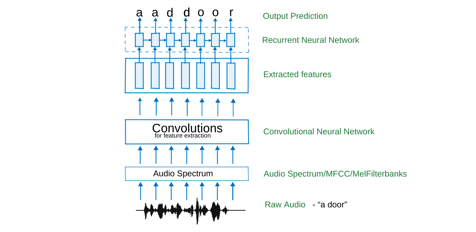
<p><img src="/images/ctc_loss/speech_model.png" alt="speech model using ctc ctc" /></p>

<p>In the model above, we convert the raw audio signal into its spectrum or apply melfiterbanks (this is optional and can be performed by a CNN layer), which is then passed through a convolution neural network (CNN). CNNs enable us extract features, by looking at a window of the data while performing strided convolutions along the feature dimension of the audio.</p>

<p>The features are then passed through a Recurrent Neural Network (RNN) for decoding. At the decoding stage, if we perform a max decoding at each timestep, we will get tokens of a much longer length than the input, which naturally implies that redundant tokens will be decoded to fill up some of the timesteps. How do we contract the decoded output to represent our predictions? How should we deal with silences in the audio? How should we indicate repetitions of tokens as in “d-oo-r”?</p>

<p>Well, Instead of decoding characters, we can decode phonemes, subwords, or even words depending on the task. Let’s consider the instance of character decoding for this article.</p>

<p>We can solve these problems by explicitly introducing a blank token into our vocabulary to cater for these dynamics. We further include a separator token to indicate spaces between each word.</p>

<p>Thus, “a door” split into [“ε”, “a”, “_”, “d”, “o”, “o”, “r”] tokens is then transformed into [“ε”, “a”, “ε”, “_”, “ε”, “d”, “ε”, “o”, “ε”, “o”, “ε”, “r”, “ε”] where the blank token is included. With this, we know that we can only have repeating tokens only if they are separated by a blank token, “ε” e.g. “d”, “o”, “ε”, “o”, “ε”, “r” is allowed and not “d”, “o”, “o”, “ε”, “r”. The latter contracts into “dor”.</p>

<p>In general, given an initial sequence of length \(M\), the length of the expanded sequence is \(2M + 1\)</p>

<h2 id="getting-into-ctc-details">Getting into ctc details</h2>

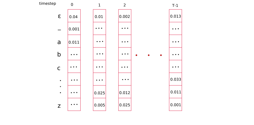
<p>At the output of the RNN, we get a vector, which has the length of vocabulary, for each time step of RNN computation. The softmax function is applied to it to get a vector of probabilities. The number of output labels cannot be more than the number of features from the CNN, so the features has to be estimated accordingly (by taking the maximum length of sequence in vocabulary or some other heuristic).</p>

<p>We will consider a smaller label “door” which should be enough to explain the entire concept succinctly. Let’s generate our vocabulary as the standard lowercase alphabets, including our special tokens.</p>

<p>[“ε”:0, “_“:1, “a”: 2, “b”:3, … ,”z”:28]</p>

<p><img src="/images/ctc_loss/softmax_layer_from_ctc.png" alt="softmax layer from ctc" /></p>

<p>We denote the total number of timesteps by \(T\), length of the expanded target output by \(S\), and length of label by \(M\). So, \(S = 2M + 1\), e.g. for “door”, \(S = 2 \cdot 4 + 1\)</p>

<p>Given these vectors of probability distributions, how do we learn the alignments of the probable predictions? We need a structured way to traverse from the first softmax distribution to the last to represent the word.</p>

<h3 id="setting-up-constrains-on-the-alignment">Setting up constrains on the alignment</h3>

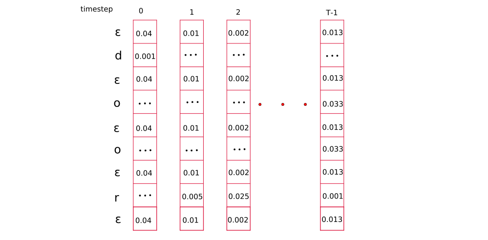
<p>In principle, we exclude all rows that do not include tokens from the target sequence and then rearrange the tokens to form the output sequence. This is done during training only. At inference, a beam search can be performed on the distribution. So, we copy the required output for the target into a secondary reduced structure and decode on the reduced structure assuring us that only appropriate tokens will be used for selected for computing loss and gradients.</p>

<p>If a token occur multiple times in the label, we repeat the rows for similar tokens in their appropriate location. This becomes our probability matrix, \(y_{(s, t)}\)</p>

<p><img src="/images/ctc_loss/reduced_softmax_layer_extract_ctc.png" alt="reduced softmax layer ctc" /></p>

<h3 id="composing-the-graph">Composing the graph</h3>

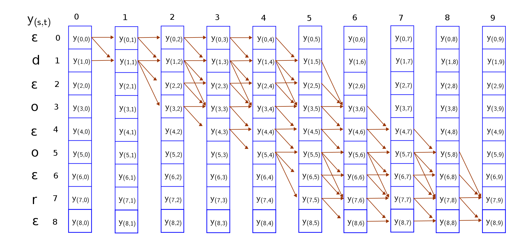
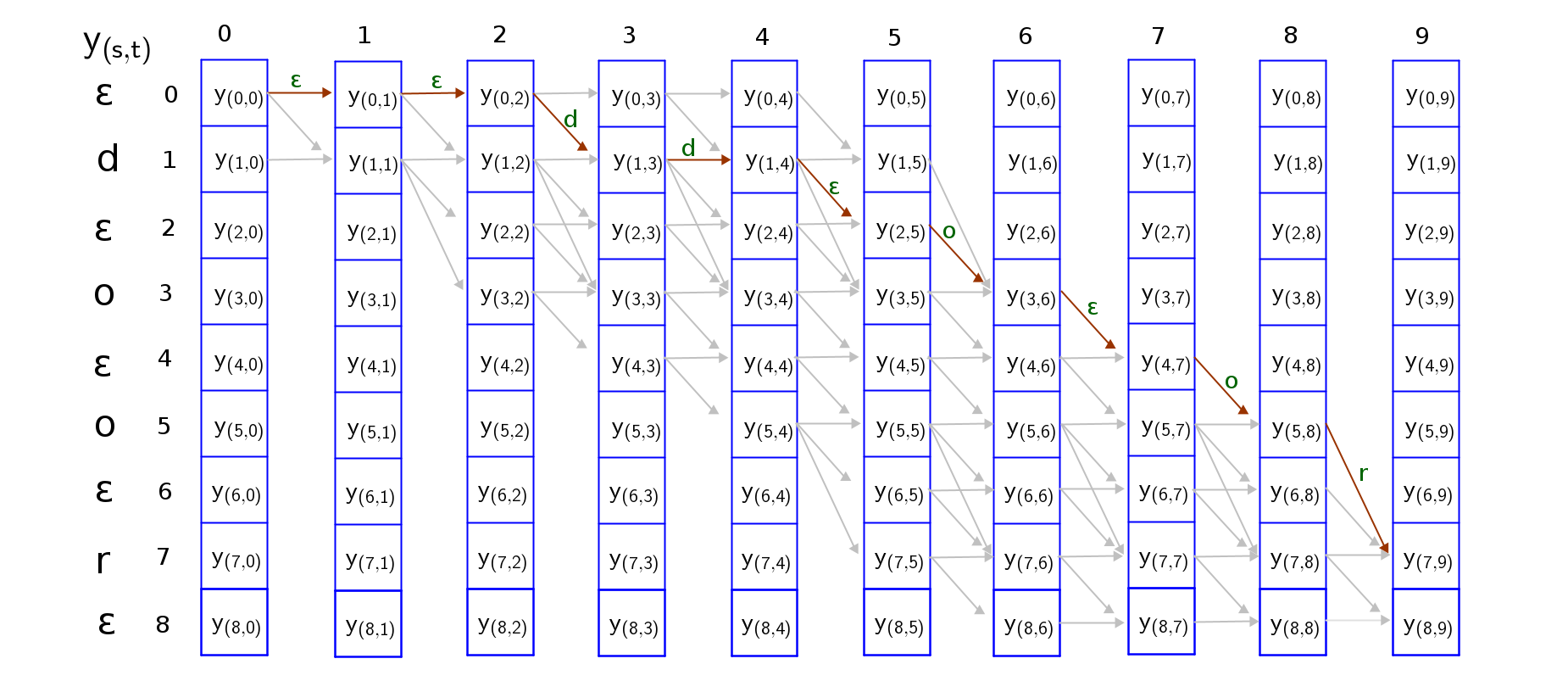
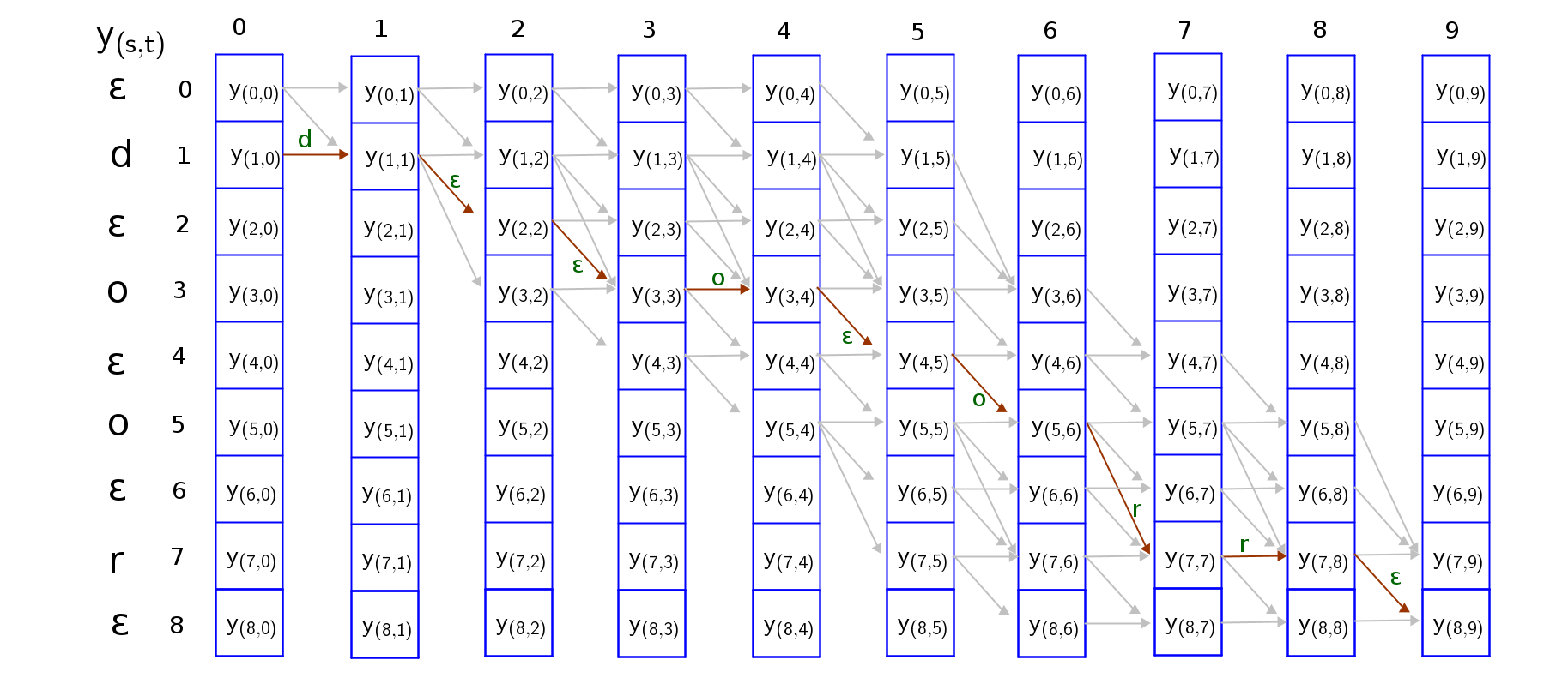
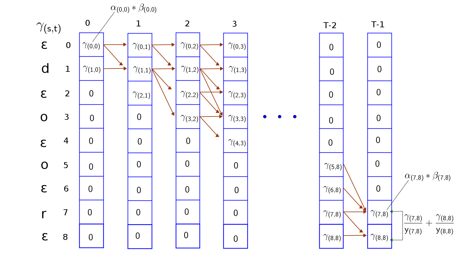
<p>Now that we have our full grid, we can begin traversing the grid from top-left to bottom right in such a way that; (a) the first character in the decoding must be a blank token, ‘ε’ or the first sequence token ‘d’ (b) the last token is either a blank token or the last sequence token ‘r’ (c) the rest of the sequence follows a sequence path that monotonically travels down from the top-left to bottom-right.</p>

<p><img src="/images/ctc_loss/probability_matrix_ctc.png" alt="probability matrix ctc" /></p>

<p>To guarantee that the sequence is an expansion of the target sequence, we can only traverse the grid through these valid paths from top-left to bottom-right. I have attempted to trave all paths in the grid, and you can do it as an exercise too. Two valid paths where both collapse into “door” are shown below;</p>

<p><img src="/images/ctc_loss/valid_paths_prob1.png" alt="ctc valid path 1" /></p>

<p><img src="/images/ctc_loss/valid_paths_prob2.png" alt="ctc valid path 2" /></p>

<p>It is easy to trace these paths if we consider the following traversal rules;</p>

<ul>
  <li>The sequence can start with a blank token or the first character token and end with a blank token or the last character token. So we have to consider both paths.</li>
  <li>Skips are permitted across a blank token <strong>only if the tokens on either side of the blank token are different</strong> because a blank is required to distinguish repetition of a token but not required between distinct tokens</li>
</ul>

<h3 id="scoring-the-paths">Scoring the paths</h3>

<p>The score of a path is the product of probabilities of all nodes along the path. For the two paths considered in the examples above.</p>

\[\begin{aligned}
\operatorname{score}(\text{path A}) &amp;= y_{(0,0)} \cdot y_{(0,1)} \cdot y_{(0,2)} \cdot y_{(1,3)} \cdot y_{(1,4)} \cdot y_{(2,5)} \cdot y_{(3,6)} \cdot y_{(4,7)} \cdot y_{(5,8)} \cdot y_{(7,9)} \\
\operatorname{score}(\text{path B}) &amp;= y_{(1,0)} \cdot y_{(1,1)} \cdot y_{(2,2)} \cdot y_{(3,3)} \cdot y_{(3,4)} \cdot y_{(4,5)} \cdot y_{(5,6)} \cdot y_{(7,7)} \cdot y_{(7,8)} \cdot y_{(8,9)}
\end{aligned}\]

<p>We are required to trace out all the possible paths that contract into “door” and there are an exponential number of such valid paths as can be seen from the graph. The complexity is of the order \(\mathcal{O}(\lvert V \rvert^T)\) where \(\lvert V \rvert\) is the length of vocabulary.</p>

<p>Can we find a dynamic programming algorithm for solving this problem? Well, the <a href="https://en.wikipedia.org/wiki/Viterbi_algorithm">viterbi algorithm</a> can generate the most likely path, and does not guarantee we get the most likely sequence of labels. It finds the best path to a node by extending the best path to one of its parent nodes. Any other path would necessarily have a lower probability. But, the viterbi algorithm commits to a path or initial alignment early (without exploration) which can lead to suboptimal results.</p>

<h2 id="forward-backward-algorithm">Forward-Backward Algorithm</h2>

<p>Instead of only selecting the most likely alignment, we find the expectation over all possible alignments during training. This allows us to also exploit the existence of subpaths in the graph.</p>

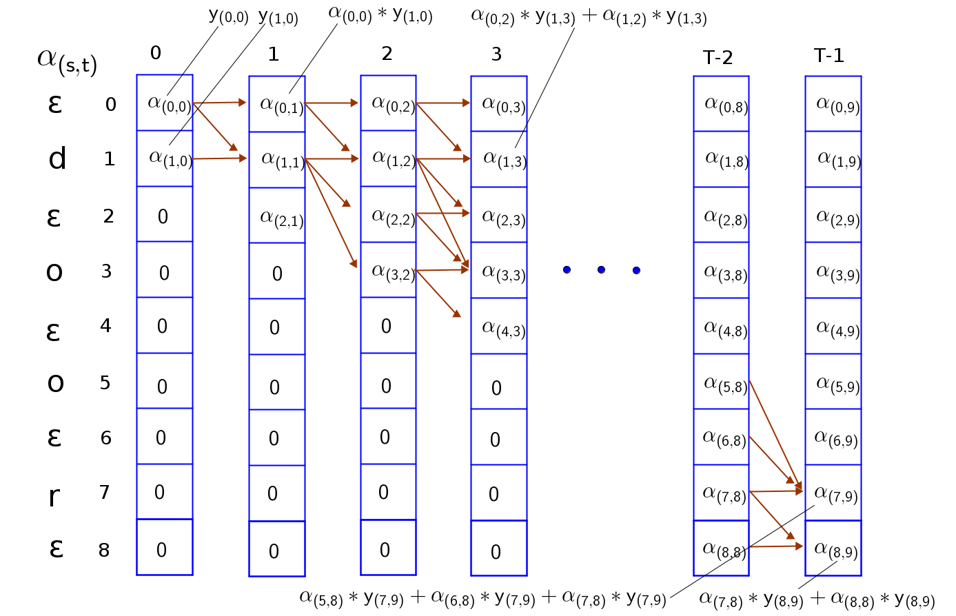
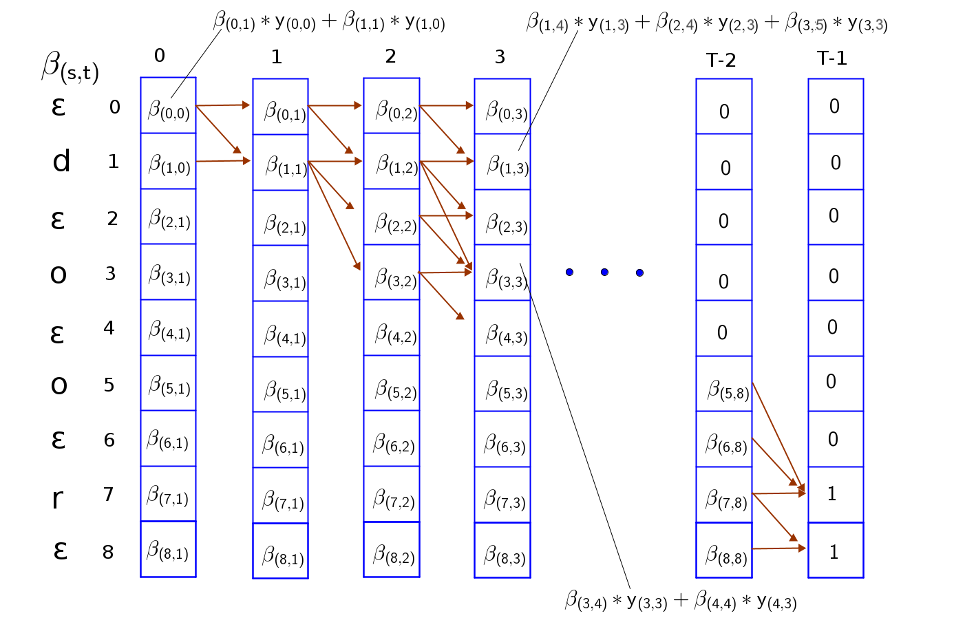
<p>To compute this effectively, we need a forward variable \(\alpha_{(s, t)}\) and backward variable \(\beta_{(s, t)}\) where \(s\) is the index of the token considered. The forward variable computes the total probability of a sequence \(\operatorname{seq}[1:s]\) up to a particular timestep \(t\). The backward variable calculates the total probability of remaining sequence from token \(\operatorname{seq}(s)\) to token \(\operatorname{seq}(S)\), \(\operatorname{seq}[s:S]\) at timestep \(t\).</p>

<h3 id="forward-algorithm-for-computing-alpha_s-t">Forward Algorithm for computing \(\alpha_{(s, t)}\)</h3>

<p>First, let’s create a matrix of zeros of same shape as our probability matrix, \(y_{(s, t)}\) to store our \(\alpha\) values. The forward algorithm is given by;</p>

<p>Initialize:</p>

<p><code class="language-plaintext highlighter-rouge">alpha_mat = zeros_like(y_mat)</code></p>

<p>\(\alpha_{(0, 0)} = y_{(0, 0)}\), \(\alpha_{(1, 0)} = y_{(1, 0)}\)</p>

<p>\(\alpha_{(s, 0)} = 0\) for \(s &gt; 1\)</p>

<p>Iterate forward:</p>

<ul>
  <li>for \(t = 1\) to \(T-1\):
    <ul>
      <li>for \(s = 0\) to \(S\):
        <ul>
          <li>\(\alpha_{(s, t)} = (\alpha_{(s, t-1)} + \alpha_{(s-1, t-1)})y_{(s, t)}\)
if \(\operatorname{seq}(s) = \text{“ε”}\) or \(\operatorname{seq}(s) = \operatorname{seq}(s-2)\)</li>
          <li>\(\alpha_{(s, t)} = (\alpha_{(s, t-1)} + \alpha_{(s-1, t-1)} + \alpha_{(s-2, t-2)})y_{(s, t)}\) otherwise</li>
        </ul>
      </li>
    </ul>
  </li>
</ul>

<p>Note that \(\alpha_{(s, t)} = 0\) for all \(s &lt; S-2(T-t) - 1\) which corresponds to the unconnected boxes in the top-right. These variables correspond to states for which there are not enough time-steps left to complete the sequence.</p>

<p>\(\operatorname{seq}(s)\) - token at index \(s\) e.g. \(\operatorname{seq}(s=1)=\text{“d”}\)</p>

<p><img src="/images/ctc_loss/alpha_prob.png" alt="computations of alpha probabilities" /></p>

<h3 id="backward-algorithm-for-computing-beta_s-t">Backward algorithm for computing \(\beta_{(s, t)}\)</h3>

<p>Let’s also create a matrix of zeros of same shape as our probability matrix, \(y_{(s, t)}\) to store our \(\beta\) values.</p>

<p>Initialize:</p>

<ul>
  <li>\(\beta_{(S-1, T-1)} = 1\), \(\beta_{(S-2, T-1)} = 1\),</li>
  <li>\(\beta_{(s, T-1)} = 0\) for \(s &lt; S-2\)</li>
</ul>

<p>Iterate backward:</p>

<ul>
  <li>for \(t = T-2\) to \(0\):
    <ul>
      <li>for \(s = S-1\) to \(0\):
        <ul>
          <li>\(\beta_{(s, t)} = \beta_{(s, t+1)}y_{(s, t)} + \beta_{(s+1, t+1)}y_{(s+1, t)}\)
if \(\operatorname{seq}(s) = \text{“ε”}\) or \(\operatorname{seq}(s) = \operatorname{seq}(s+2)\)</li>
          <li>\(\beta_{(s, t)} = \beta_{(s, t+1)}y_{(s, t)} + \beta_{(s+1, t+1)}y_{(s+1, t)} + \beta_{(s+2, t+2)}y_{(s+2, t)}\) otherwise</li>
        </ul>
      </li>
    </ul>
  </li>
</ul>

<p>Similarly, \(\beta_{(s, t)} = 0\) for all \(s &gt; 2t\) which corresponds to the unconnected boxes in the bottom-left.</p>

<p><img src="/images/ctc_loss/beta_prob.png" alt="computations of beta probabilities" /></p>

<h3 id="computing-the-probabilities-efficiently">Computing the probabilities efficiently</h3>

<p>From the computations, observe that we are constantly multiplying values less than 1. This can lead to underflow especially for longer sequences. We can improve these computations by performing the computations in the logarithm space. Products become sums, divisions become subtraction. For instance;</p>

\[\alpha_{s, t} = (\alpha_{s, t-1} + \alpha_{(s-1, t-1)})y_{s, t}\]

<p>becomes</p>

\[\log \alpha_{s,t} = \log( e^{\log\alpha_{s,t-1}} + e^{\log\alpha_{s-1,t-1}}) + \log P_{s,t}\]

<h3 id="ctc-loss-calculation-for-each-timestep">CTC Loss calculation for each timestep</h3>

<p>Now that we have the \(\alpha\) and \(\beta\) probabilities(or log probabilities), we will compute the joint probability of the sequence at every timestep. This we will call \(\gamma_{s,t}\).</p>

\[\gamma_{s,t} = \alpha_{s,t}\beta_{s,t}\]

<p>Afterwards, we compute the posterior probabilities of the sequence at every timestep by summing along columns. This is the total probability of all paths going through a token \(\operatorname{seq}(s)\) at timestep t.</p>

\[P_{(\operatorname{seq}_t, t)} = \sum\limits_{s=0}^{S}\dfrac{\alpha_{s,t}\beta_{s,t}}{y_{s,t}}\]

<p><img src="/images/ctc_loss/gamma_prob.png" alt="computations of gamma probabilities" /></p>

<p>Total loss of the model is then;</p>

\[\mathcal{L} = -\sum\limits_{t=0}^{T-1} \log P_{(\operatorname{seq}_t, t)}\]

<p>Derivatives can then be calculated for back propagation using Autograd. Modern deep leaning libraries such as Pytorch, and TensorFlow have this feature.</p>

<h3 id="note">Note</h3>

<ol>
  <li>The CTC loss algorithm can be applied to both convolutional and recurrent networks. For recurrent networks, it is possible to compute the loss at each timestep in the path or make use of the final loss, depending on the use case.</li>
  <li>Some forms of the loss use only the forward algorithm in its computation i.e \(\alpha_{s, t}\). I was only able to reproduce the Pytorch CTC loss when I used the forward algorithm in my loss computation, and ignoring the backward algorithm. However, the algorithm explained in this blog post is the one proposed in the seminal paper by Graves et al.<d-cite key="graves2006ctc"></d-cite>.</li>
</ol>

<h2 id="conclusion">Conclusion</h2>

<p>In this article, we explained the connectionist temporal classification loss and how it can be applied in many-to-many input/output classification tasks without alignments. Then, we showed the computations for the forward and backward algorithm used for the training the model.</p>]]></content><author><name>Sewade Ogun</name><email>sogun@aimsammi.org</email></author><category term="blog" /><category term="loss" /><summary type="html"><![CDATA[How the forward-backward algorithm computes the Connectionist Temporal Classification loss, step by step.]]></summary></entry><entry><title type="html">From GRU to Transformer</title><link href="https://ogunlao.github.io/blog/2020/06/12/from_gru_to_transformer.html" rel="alternate" type="text/html" title="From GRU to Transformer" /><published>2020-06-12T00:00:00+00:00</published><updated>2020-06-12T00:00:00+00:00</updated><id>https://ogunlao.github.io/blog/2020/06/12/from_gru_to_transformer</id><content type="html" xml:base="https://ogunlao.github.io/blog/2020/06/12/from_gru_to_transformer.html"><![CDATA[<p>Attention-based networks have been shown to outperform recurrent neural networks and its variants for various deep learning tasks including Machine Translation, Speech, and even Visio-Linguistic tasks. The Transformer <a href="https://papers.nips.cc/paper/7181-attention-is-all-you-need.pdf">[Vaswani et. al., 2017]</a> is a model, at the fore-front of using only self-attention in its architecture, avoiding recurrence and enabling parallel computations.</p>

<p>To understand how the self-attention mechanism is applied in Transformers, it might be intuitive from a mathematical perspective to build-up step-by-step from what is known, i.e. Recurrent Neural Networks such as LSTMs or GRUs to a self-attention network such as Transformers. Blog posts such as <a href="https://jalammar.github.io/illustrated-transformer/">Jalammar</a>, <a href="http://nlp.seas.harvard.edu/2018/04/03/attention.html">The Annotated Transformer</a>, <a href="http://vandergoten.ai/2018-09-18-attention-is-all-you-need/">Vandergoten</a> have attacked the explanation of Transformers from different perspectives but I believe this article will give another perspective and help engineers and researchers understand Self-Attention better, as I did.</p>

<p>For a beautiful explanation of everything Attention, check out <a href="https://lilianweng.github.io/lil-log/2018/06/24/attention-attention.html">Lilianweng post on Attention</a></p>

<p>Here’s what we will cover:</p>
<ol id="markdown-toc">
  <li><a href="#introduction" id="markdown-toc-introduction">Introduction</a></li>
  <li><a href="#gated-recurrent-neural-networks" id="markdown-toc-gated-recurrent-neural-networks">Gated Recurrent Neural Networks</a>    <ol>
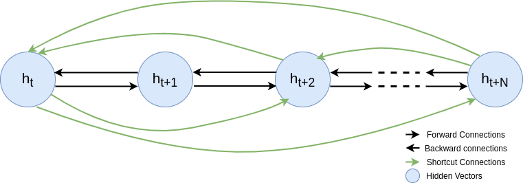
      <li><a href="#what-are-these-shortcut-connections" id="markdown-toc-what-are-these-shortcut-connections">What are these shortcut connections</a></li>
    </ol>
  </li>
  <li><a href="#gated-recurrent-units-to-causal-attention" id="markdown-toc-gated-recurrent-units-to-causal-attention">Gated Recurrent Units to Causal Attention</a>    <ol>
      <li><a href="#lets-free-the--dependent-weights" id="markdown-toc-lets-free-the--dependent-weights">Let’s free the  dependent weights</a></li>
      <li><a href="#lets-free-up-candidate-vectors" id="markdown-toc-lets-free-up-candidate-vectors">Let’s free up candidate vectors</a></li>
      <li><a href="#lets-separate-keys-and-values" id="markdown-toc-lets-separate-keys-and-values">Let’s separate Keys and Values</a></li>
      <li><a href="#lets-have-multiple-attention-heads" id="markdown-toc-lets-have-multiple-attention-heads">Let’s have multiple attention heads</a></li>
    </ol>
  </li>
  <li><a href="#gated-recurrent-units-to-non-causal-attention" id="markdown-toc-gated-recurrent-units-to-non-causal-attention">Gated Recurrent Units to Non-Causal Attention</a>    <ol>
      <li><a href="#lets-look-at-the-entire-input-sequence" id="markdown-toc-lets-look-at-the-entire-input-sequence">Let’s look at the entire input sequence</a></li>
      <li><a href="#lets-give-a-sense-of-position-to-the-attention-mechanism" id="markdown-toc-lets-give-a-sense-of-position-to-the-attention-mechanism">Let’s give a sense of position to the attention mechanism</a></li>
      <li><a href="#lets-use-non-linear-attention" id="markdown-toc-lets-use-non-linear-attention">Let’s use Non-Linear Attention</a></li>
    </ol>
  </li>
  <li><a href="#full-self-attention-layer" id="markdown-toc-full-self-attention-layer">Full Self-Attention Layer</a></li>
  <li><a href="#conclusion" id="markdown-toc-conclusion">Conclusion</a></li>
</ol>

<p>This article is based on a lecture given by <a href="https://kyunghyuncho.me/">Kyunghyun Cho</a> at AMMI, 2020. Special thanks to him and his team for a beautiful NLP course.</p>

<h2 id="introduction">Introduction</h2>

<p>Recurrent neural networks with gates such as Long-Short Term Memory (LSTM) and Gated Recurrent Units (GRU) have long been used for sequence modelling with the advantage that they help to significantly solve the vanishing problem and long-term dependency problems popularly found in Vanilla RNNs. Attention mechanisms have also been used together with these gated recurrent networks to improve their modelling capacity. However, recurrent computations still persist.</p>

<p>Given a sequence of input tokens, \((x_1, x_2, \dots, x_T)\), where T is the total number of tokens. At time step \(t\), we can calculate a hidden vector \(h_t\) which is a representation of information gotten from tokens from time step \(1\) to \(t\).</p>

<h2 id="gated-recurrent-neural-networks">Gated Recurrent Neural Networks</h2>

<p>A key idea behind LSTM and GRU is the additive update of the hidden vector, \(h_t \in \mathbb{R}^d\) with dimension, d</p>

\[h_t = u_t \odot h_{t-1} + (1 - u_t) \odot \tilde{h}_t\]

<p>where \(\tilde{h}_t\) is the candidate context vector for current time-step, \(t\) which is gated and added to the previous context vector in a linear way. This allows information to be propagated from previous time-steps to the current time step, if necessary. As observed, the update gate, \(u_t \in \mathbb{R}^d\)</p>

<ul>
  <li>With \(u_t \approx 0\) (zero vector), \(h_t = \tilde{h}_t\) implying the candidate vector represents the new context vector, \(h_t\), ignoring information from previous time-step.</li>
  <li>With \(u_t \approx 1\), (vector of 1s), \(h_t = h_{t-1}\) implying the previous context vector is copied to the new time-step, discarding the candidate vector information</li>
  <li>In  most cases, \(u_t\) will take values between \(0\) and \(1\), allowing some information depending on their values.</li>
</ul>

<p>\(\tilde{h}_t\) is a function of the current input, \(x_t\) and the previous hidden vector, \(h_{t-1}\).</p>

\[\tilde{h}_t = f(x_t, h_{t-1}) = \tanh(\textbf{W} x_t + \textbf{U}h_{t-1} + b)\]

<p>where \(\textbf{W}\), \(\textbf{U}\) are weight matrices, and \(b\) is a vector.</p>

<p>Note that we have simplified the GRU update equations ignoring the reset gate.</p>

<p>An interpretation of the additive updates is that they help to create linear shortcut connections between the hidden vectors of the current state and previous states (similar to residual connections found in popular neural network architectures such as ResNet).</p>

<p><img src="/images/short-cut_gru.png" alt="Shortcut connections between hidden vectors in GRU" title="Shortcut connections between hidden vectors in GRU" /></p>

<h3 id="what-are-these-shortcut-connections">What are these shortcut connections</h3>

<p>If we begin to unroll the hidden vector equation, moving step by step backwards, to extract the computations done to arrive there, we notice that it forms a weighted combination of all previous hidden vectors.</p>

\[\begin{aligned}
h_t &amp;= u_t \odot h_{t-1} + (1 - u_t) \odot \tilde{h}_t \\
    &amp;= u_t \odot \left(u_{t-1} \odot h_{t-2} + (1-u_{t-1}) \odot \tilde{h}_{t-1}\right) + (1-u_t) \odot \tilde{h}_t \\
    &amp;= u_t \odot \left(u_{t-1} \odot \left(u_{t-2} \odot h_{t-3} + (1-u_{t-2}) \odot \tilde{h}_{t-2} \right) + (1-u_{t-1}) \odot \tilde{h}_{t-1} \right) + (1-u_t) \odot \tilde{h}_t \\
    &amp;\;\;\vdots \\
    &amp;= \sum_{i=1}^t \left(\prod_{j=1}^{t-i+1} u_j \right) \left(\prod_{k=1}^{i-1} (1-u_k) \right) \tilde{h}_i
\end{aligned}\]

<p>for \(t\) steps of GRU update. The breakdown of \(h_t\) shows the computation involving weighted combinations of all GRU’s previous states.</p>

<h2 id="gated-recurrent-units-to-causal-attention">Gated Recurrent Units to Causal Attention</h2>

<p>In causal attention as in GRUS, we will only have access or look at previous hidden states. This will allow us to proceed with our decomposition, but will be relaxed later to give a general non-causal attention.</p>

<p>Looking at the expanded version of the GRU update, we see dependencies between a lot of parameters and components. We will attempt to free these dependencies one-by-one given rise to a disentangled unit.</p>

\[h_t = \sum_{i=1}^t \left(\prod_{j=1}^{t-i+1} u_j \right) \left(\prod_{k=1}^{i-1} (1-u_k) \right) \tilde{h}_i\]

<h3 id="lets-free-the--dependent-weights">Let’s free the  dependent weights</h3>

<p>Recall that the update gate, \(u_t\) is calculated thus in GRUs;</p>

\[\begin{aligned}
u_t &amp;= \sigma(W_x x_{t-1} + U_h h_{t-1} + b_u) \\
h_t &amp;= f(h_{t-1}, x_{t-1}) = u_t \odot \tilde{h}_t + (1-u_t)\odot h_{t-1}
\end{aligned}\]

<p>where \(W_x\), \(U_h\) are weight matrices of the Update gate computation, \(b_u\) is a bias vector and \(h_t\), \(x_t\) are hidden and input vectors respectively.</p>

<p>From both equations, we can observe that \(u_t\), the current update gate is dependent on \(h_{t-1}\), the previous hidden vector and vice-versa. To disentangle \(u_t\) from \(h_{t-1}\), we can learn the current hidden context, \(h_t\) as a weighted combination of candidate vectors, \(h_i\).</p>

\[h_t = \sum_{i=1}^t \alpha_i \tilde{h}_i\]

<p>where \(\alpha_i \propto \exp\left(\operatorname{ATT}\left(\tilde{h}_i, x_t\right)\right)\) and \(i\) ranges from time-step \(1\) to the current time-step, \(t\), implying that it uses the candidate vectors of all previous and current state to evaluate the hidden vector.</p>

<h3 id="lets-free-up-candidate-vectors">Let’s free up candidate vectors</h3>

<p>Recall that \(\tilde{h} = f(x_t, h_{t-1})\)</p>

<p>where \(\tilde{h}_t\) depends on \(h_{t-1}\); \(h_{t-1}\) depends on \(\tilde{h}_{t-1}\) and \(h_{t-2}\) and so on - check unrolled \(h_t\) above.</p>

<p>This implies that \(\tilde{h}_t\) still depends on all the previous \(\tilde{h}_{t-N}\) candidate vectors.</p>

<p>To break these dependencies in candidate vectors, \(h\),
Recall that;</p>

\[h_t = \sum_{i=1}^t \alpha_i \tilde{h}_i\]

<p>we replace the candidate vector by an input function \(f(x_i)\). This input function takes in \(x_i \in \mathbb{R}^d\) and map it into a space of \(\tilde{h}_i \in \mathbb{R}^d\), without having to explicitly use previous candidate vectors.</p>

<p>The input function \(f(x_i)\) which have been used to disentangle the candidate vectors for each time-step can serve different purposes as we see in Transformers.</p>

<ol>
  <li>
    <p>It is sometimes used to query which of the previous hidden states are important, i.e.</p>

\[\alpha_i \propto \exp\left(\operatorname{ATT}\left(f(x_i), f(x_t)\right)\right)\]

    <p>where \(i\) ranges from \(1\) to \(t\), \(f(x_i)\) represents the Key vector and \(f(x_t)\), the Query vector of the attention function, \(\operatorname{ATT}(., .)\). This attention function provides relatively high \(\alpha_i\) values for \(f(x_i)\) values associated with current token, \(f(x_t)\).</p>
  </li>
  <li>
    <p>As seen, it is also used to calculate the candidate vectors for the content update i.e.</p>

\[h_t = \sum_{i=1}^t \alpha_i f(x_i)\]

    <p>where \(f(x_i)\) serves as the Value vector here.</p>

    <p>In summary, pass in a vector of input \(x_i\) or \(x_t\) to function \(f(.)\) depending on what is required to calculate Query, Key and Value.</p>
  </li>
</ol>

<ul>
  <li>
    <p>What is \(f(x_t)\) or \(f(x_i)\) ?</p>

    <p>\(f(.)\) is a function that processes the current input \(x_t\) or previous hidden vectors, \(x_i\). At the input to the encoder or decoder, if \(x_t\) or \(x_i\) is a one-hot vector representation of a token, \(f(.)\) is a lookup table or embedding layer. If \(x_i\) is a hidden state from the lower layer, \(f(.)\) can either be an identity function or a MLP.</p>
  </li>
</ul>

<p>Even though we have performed a lot of disentanglement, notice that Key, Value and Query vectors will be similar as they are derived from the same function.</p>

<h3 id="lets-separate-keys-and-values">Let’s separate Keys and Values</h3>

<p>Instead of using a single linear function, let’s apply independent but similar linear functions to each of Keys, Values and Queries. These will just be 3 neural networks, \(K\), \(Q\), \(V\) with independent weights. So we have;</p>

<ul>
  <li>
    <p>the Key vector network, \(K\) and Query vector network, \(Q\) used in the attention function, \(\operatorname{ATT}\) to calculate the attention weights, \(\alpha_i\)</p>

\[\alpha_i \propto \exp(\operatorname{ATT}(K(f(x_i)), Q(f(x_t))))\]
  </li>
  <li>
    <p>the value vector network, \(V\) used to calculate \(h_t\),</p>

\[h_t = \sum_{i=1}^t \alpha_i V(f(x_i))\]
  </li>
</ul>

<p>Putting it another way, we compute the attention weights, \(\alpha_i\) by comparing the query vector of the current position, \(Q(f(x_t))\) against all the key vectors of the previous inputs, \(K(f(x_i))\), then compute the weighted sum of the Value vectors of all the previous inputs, \(V(.)\) to get the hidden vector, \(h_t\) at time-step \(t\).</p>

<p>At this stage, we have pretty much built a disentangled model but ehrmm, we have only a single attention mechanism. Will this be enough to model all the dependencies in context/hidden vectors? Maybe, it will be a good idea to have multiple attention heads. What do you think?</p>

<h3 id="lets-have-multiple-attention-heads">Let’s have multiple attention heads</h3>

<p>We can create N multiple possible \(Q\), \(K\) and \(V\) functions/neural networks. Since each of them takes in the same \(x_i\) or \(x_t\), we can have parallel computation performed by each \(Q\), \(K\) and \(V\) functions.</p>

<p>For each attention head, \(n \in \{1, 2, 3, \dots, N\}\), we calculate \(h_t^n\). Each \(h_t^n\) is concatenated together to form the new \(h_t\) i.e.</p>

\[h_t = \left[h_t^1;~ h_t^2;~ \dots;~ h_t^N \right]\]

<p>where</p>

<p>\(h_t^n = \sum_{i=1}^t \alpha_i^n V^n(f(x_i))\) and \(\alpha_i^n \propto \exp(\operatorname{ATT}(K^n(f(x_i)), Q^n(f(x_t))))\)</p>

<p>Questions?</p>

<ul>
  <li>Why concatenate the multiple attention heads instead of adding them, or use some other methods?
Well, the concatenation gives a vector with a representation that provides information about different aspects of the inputs, and allows each head to specialize in attending. I don’t have an answer for that, if you do, please leave it in the comment section.</li>
</ul>

<h2 id="gated-recurrent-units-to-non-causal-attention">Gated Recurrent Units to Non-Causal Attention</h2>

<p>We have previously only attended to previous and current hidden states in our network. In non-causal attention, we relax this assumption and we are allowed to also look at positions \(t+1\) to \(T\) of the sequence.</p>

<h3 id="lets-look-at-the-entire-input-sequence">Let’s look at the entire input sequence</h3>

<p>Since we have broken all the dependencies of candidate vectors and attention weights of all hidden states from \(t = 1, \dots, T\), at time-step/position, \(t\), we can utilize the previous hidden states, current hidden state as well as future hidden states. I prefer to call \(t\) position now that there are no recurrent computations really.</p>

<p>\(h_t\) then becomes;</p>

\[h_t = \left[h_t^1;~ h_t^2;~ \dots;~ h_t^N \right]\]

<p>where \(h_t^n = \sum_{i=1}^T \alpha_i^n V^n(f(x_i))\)</p>

<p>and \(\alpha_i^n \propto \exp(\operatorname{ATT}(K^n(f(x_i)), Q^n(f(x_t))))\)</p>

<p>Great!!, now we have a more robust attention mechanism. One problem still persists though. With this mechanism, we can just permute the order of the hidden states and nothing changes. Is that the behavior we want? Hmm, No!</p>

<h3 id="lets-give-a-sense-of-position-to-the-attention-mechanism">Let’s give a sense of position to the attention mechanism</h3>

<p>We can do this by adding a position encoded vector, \(p(i)\) (usually of same dimension) to each input. Each \(p(i)\) comes from a positional embedding \(p\). This positional embedding is independent of the actual token embeddings.</p>

<p>So \(h_t\) becomes;</p>

\[h_t = \left[h_t^1;~ h_t^2;~ \dots;~ h_t^N \right]\]

<p>where</p>

\[h_t^n = \sum_{i=1}^T \alpha_i^n V^n(f(x_i) + p(i))\]

<p>and \(\alpha_i^n \propto \exp(\operatorname{ATT}(K^n(f(x_i)), Q^n(f(x_t) + p(i))))\)</p>

<p>\(p(i)\) is the position encoded vector for position \(i\) from positional embedding \(p\).</p>

<p>Learned positional embedding and function-based positional embedding (such as sinusoidal positional embedding) are the common positional embeddings. The Transformer uses the sinusoidal positional embedding due to the property that it can generalize to lengths not seen during training.</p>

<p>To this point, we have only been using linear projections as our functions. Do you think a sprinkle of non-linearity will help our model?</p>

<h3 id="lets-use-non-linear-attention">Let’s use Non-Linear Attention</h3>

<p>As seen from our discussion, we can extract the following about the linearity of our Attention.
With</p>

\[h_t^n = \sum_{i=1}^T \alpha_i^n V^n(f(x_i) + p(i))\]

<ul>
  <li>the hidden vectors calculated through attention are inherently linear and are just weighted sum of input vectors.</li>
  <li>Also, \(f(.)\) is often an identity function (especially for intermediate layers)</li>
  <li>p, the positional embedding does not depend on the input.</li>
  <li>the Values vector network, V is often a linear transformation.</li>
</ul>

<p>With the following observations, it will be difficult for the attention to manipulate the attention weights to find a complicated combination. The solution will be to apply a post-attention non-linear function.</p>

<p>Let’s define \(g(.)\) as the post-attention non-linear function, which is a feed-forward neural network in our case, applied to each time-step independently.</p>

\[h_t = g\left(\left[h_t^1;~ h_t^2;~ \dots;~ h_t^N \right]\right)\]

<p>For higher efficiency, \(g\) may be applied to each head independently. \(h_t\) becomes;</p>

\[h_t = \left[g(h_t^1);~ g(h_t^2);~ \dots;~ g(h_t^N) \right]\]

<p>This gives us the <strong>Non-Linear, Non-Causal, Positional Attention</strong> used by Transformer.</p>

<p>It has been a long ride. If you have got this far, you are a Genius!! You must have gotten something from the article. Let’s bring all together in one place.</p>

<h2 id="full-self-attention-layer">Full Self-Attention Layer</h2>

<p>In summary,</p>

<ul>
  <li>
    <p>the context vector with a single attention mechanism is calculated thus;</p>

\[h_t^n = \sum_{i=1}^T \alpha_i^n V^n(f(x_i) + p(i))\]
  </li>
  <li>
    <p>which are then concatenated together, either before or after applying a nonlinear function</p>

\[h_t = g\left(\left[h_t^1;~ h_t^2;~ \dots;~ h_t^N \right]\right)\]

    <p>or</p>

\[h_t = \left[g(h_t^1);~ g(h_t^2);~ \dots;~ g(h_t^N) \right]\]
  </li>
  <li>
    <p>then, the attention weight are calculated using the Key and Query vectors as well as positional encoding for the input</p>

\[\alpha_i^n \propto \exp(\operatorname{ATT}(K^n(f(x_i) + p(i)), Q^n(f(x_t) + p(i))))\]
  </li>
</ul>

<h2 id="conclusion">Conclusion</h2>

<p>In this article, we showed how we can move from a recurrent-based neural network with gates such as GRU to a self-attention based model such as Transformer with disentangled hidden states and weights, enabling parallel computations.</p>]]></content><author><name>Sewade Ogun</name><email>sogun@aimsammi.org</email></author><category term="blog" /><category term="GRU" /><category term="attention" /><category term="neural_network" /><summary type="html"><![CDATA[Attention-based networks have been shown to outperform recurrent neural networks and its variants for various deep learning tasks including Machine Translation, Speech, and even Visio-Linguistic tasks. The Transformer [Vaswani et. al., 2017] is a model, at the fore-front of using only self-attention in its architecture, avoiding recurrence and enabling parallel computations.]]></summary></entry><entry><title type="html">K Nearest Neighbor as a Neural Network</title><link href="https://ogunlao.github.io/2020/05/23/knn-as-a-neural-network.html" rel="alternate" type="text/html" title="K Nearest Neighbor as a Neural Network" /><published>2020-05-23T00:00:00+00:00</published><updated>2020-05-23T00:00:00+00:00</updated><id>https://ogunlao.github.io/2020/05/23/knn-as-a-neural-network</id><content type="html" xml:base="https://ogunlao.github.io/2020/05/23/knn-as-a-neural-network.html"><![CDATA[<p>A Neural network is a universal function approximator, so in theory it is possible to learn any function using a neural network. As K-nearest neighbor is a method of predicting the label of a new datapoint from the test set, it is possible to express its prediction function as a neural network, although less intuitive. This article will show how to express a 1-Nearest Neighbor as a 3 layer neural network, using the given datapoints. If you will like to jump directly into the accompanying code, just <a href="https://github.com/ogunlao/ogunlao.github.io/blob/master/notebooks/knn_as_neural_network.ipynb">follow this link</a> to the notebook.</p>

<p>Here’s what we will cover:</p>
<ol id="markdown-toc">
  <li><a href="#introduction" id="markdown-toc-introduction">Introduction</a></li>
  <li><a href="#k-nearest-neighbor" id="markdown-toc-k-nearest-neighbor">K Nearest Neighbor</a></li>
  <li><a href="#expressing-knn-as-a-neural-network" id="markdown-toc-expressing-knn-as-a-neural-network">Expressing KNN as a Neural Network</a>    <ol>
      <li><a href="#layer-1-computing-the-distance-function" id="markdown-toc-layer-1-computing-the-distance-function">Layer 1: Computing the distance function</a></li>
      <li><a href="#layer-2-softmax-layer" id="markdown-toc-layer-2-softmax-layer">Layer 2: Softmax Layer</a></li>
      <li><a href="#layer-3-prediction-layer" id="markdown-toc-layer-3-prediction-layer">Layer 3: Prediction Layer</a></li>
    </ol>
  </li>
  <li><a href="#implementation" id="markdown-toc-implementation">Implementation</a></li>
  <li><a href="#future-work" id="markdown-toc-future-work">Future Work</a></li>
  <li><a href="#conclusion" id="markdown-toc-conclusion">Conclusion</a></li>
  <li><a href="#reference" id="markdown-toc-reference">Reference</a></li>
</ol>

<h2 id="introduction">Introduction</h2>

<p>k-Nearest Neighbor is a non-parametric model that uses a distance function to evaluate the label of a new test point. It involves taking the average of predictions of k nearest points to the given test point. It often serves a base model for many predictions tasks and often difficult to beat.</p>

<p>Given a set of train data-points,</p>

\[\{(x_1, y_1), (x_2, y_2), \dots ,(x_n, y_n)\}\]

<p>with \(x_i \in \mathbb{R}^d\), \(y_i \in \mathbb{R}\) and \(i = 1, 2, \dots, n\). There are \(n\) training examples each with d number of features. Given a new datapoint \(x^t\), how can we classify the point using k-nearest neighbor into its correct class?</p>

<h2 id="k-nearest-neighbor">K Nearest Neighbor</h2>

<p>To classify a new test point into its correct label, we perform the following steps:</p>

<ul>
  <li>Calculate the distance between each datapoint in the training example and the test datapoint</li>
  <li>Assign the test data point the label of the k datapoints with minimum distance. for a classification task, we can take the mode of the k classes, while for regressing task, we average the predictions to get the prediction.</li>
  <li>k can range from 1 to n, but usually between 1 and 10.</li>
  <li>The distance function takes in each \(x_i\) and \(x^t\) and outputs a scalar. The distance function to use may depend on the task but a popular and common distance is the l2-distance. The l2-distance can be expressed as:</li>
</ul>

\[d_i = \sqrt{\sum_{j=1}^{d} (x_{ij} - x^t_j)^2}\]

<p>Using the matrix notation,</p>

\[d = \sqrt{\sum_{j=1}^{d} (X_j^2 - 1_n(x^t)_j^T)^2}\]

<p>where \(X = (x_1, x_2, \dots, x_n)^T \in \mathbb{R}^{n \times d}\) and \((x^t)^T \in \mathbb{R}^d\). To simplify notation, I will assume that \(x^t\) will be broadcasted along the matrix, which becomes simply:</p>

\[d = \sqrt{\sum_{j=1}^{d} (X_j^2 - x_j^t)^2}\]

<h2 id="expressing-knn-as-a-neural-network">Expressing KNN as a Neural Network</h2>

<p>With the understanding of the distance function, we can break it apart to derive the parameters of our neural network.</p>

<p>From the distance function,</p>

\[d_i^2 = \sum_{j=1}^{d} (x_{ij} - x_j)^2 = d'\]

<p>Since optimizing \(d^2\) is equivalent to optimizing for \(d\), we work with \(d^2\) instead, which we will call \(d'\)</p>

<h3 id="layer-1-computing-the-distance-function">Layer 1: Computing the distance function</h3>

<p>Expanding the equation, we get:</p>

\[d' = \sum_{j=1}^{d} \left((X^2_j - x^t_j) \odot (X^2_j - x^t_j)\right)\]

<p>Note that: \(\odot\) is a hadamard product, i.e. element-wise product between the two matrices.</p>

\[\begin{aligned}
d' &amp;= \sum_{j=1}^{d} \left(X^2_j + (x^t_j)^2 - 2X_j \cdot x^t\right) \\
     &amp;= -2X_jx^t + \sum_{j=1}^{d} \left(X^2_j + (x^t_j)^2\right)
\end{aligned}\]

<p>since the \(-2X_jx^t\) does not depend on j.</p>

<p>At this point we can easily extract our first layer, \(Z_1 = W_1x_1 + b\) where \(W_1 = -2X_j\), \(x_1 = x^t\) and \(b = \sum_{j=1}^{d} \left(X^2_j + (x^t_j)^2\right)\)</p>

<h3 id="layer-2-softmax-layer">Layer 2: Softmax Layer</h3>

<p>After the previous step, we then need to find the datapoint with the closest distance to the test datapoint. This can be performed in two steps using the softmax layer:</p>

<ul>
  <li>Negate the vector, so the datapoint with minimum distance, then have the maximum value.</li>
  <li>Multiply the vector by a large positive constant \(\lambda \rightarrow \infty\). This has the effect of shrinking small values and increases already large values. The intention is to have the neuron turned on for only the minimum value of the input \(Z_1\). This is equivalent to applying the softmax temperature on the vector. \(\lambda\) is an hyperparameter.</li>
</ul>

\[Z_2 = softmax(-\lambda * Z_1)\]

<blockquote>
  <p>For a refresher on the softmax temperature, check my previous post on <a href="https://ogunlao.github.io/2020/04/26/you_dont_really_know_softmax.html#softmax-temperature">Softmax temperature</a></p>
</blockquote>

<h3 id="layer-3-prediction-layer">Layer 3: Prediction Layer</h3>

<p>Before now, we have not really talked out the labels of the training examples. It comes in at this layer to support in prediction.</p>

<ul>
  <li>For a regression task, this computation is almost done. We take the vector of distances and find the prediction of the class, with the minimum distance (or maximum value in this case, as we have performed inversion).</li>
  <li>For a classification task, we can also take the label of the datapoint with the minimum distance or go a step further.</li>
</ul>

<p>For a classification task, where \(Z_3 = W_3x_3 + b\), firstly, we perform one-hot encoding on the train labels. \(y_{\text{onehot}} \in \mathbb{R}^{n \times d}\)</p>

\[Z_3 = Z_2^Ty_{\text{onehot}}\]

<p>where \(W_3 = X^T\), \(x_3 = z_2\), \(b = 0\)</p>

<h2 id="implementation">Implementation</h2>

<p>I created a jupyter notebook to show predictions on the iris dataset. You can access the notebook <a href="https://github.com/ogunlao/ogunlao.github.io/blob/master/notebooks/knn_as_neural_network.ipynb">via this link</a>. Feel free to drop comments, and possibly give area for clarification or improvement. Let me try to explain the major parts of the implementation.</p>

<ul>
  <li>Data: Loaded the iris dataset via the sklearn load dataset api.</li>
  <li>Preprocessing: Normalized the dataset (often a good thing to normalize) and converted each label into one-hot encoded vectors.</li>
  <li>Built a 3 layer neural network using the datapoints as parameters.</li>
</ul>

<h2 id="future-work">Future Work</h2>

<p>A 1-Nearest Neighbor implementation was discussed here. This can be extended to k- nearest neighbors. How will you go about it?</p>

<h2 id="conclusion">Conclusion</h2>

<p>In this article, We showed how a k-nearest neighbor classifier can be transformed into a neural network using the datapoints as parameters. This is also a non-parametric model and the weights of the model increases as the number of training points increases. Finally, neural network is a universal function approximator and can therefore be an exercise to represent other models in terms of a basic neural network model.</p>

<hr />

<h2 id="reference">Reference</h2>

<ol>
  <li>Yan Qiu Chen, R. I. Damper and M. S. Nixon, “On neural-network implementations of k-nearest neighbor pattern classifiers,” in IEEE Transactions on Circuits and Systems I: Fundamental Theory and Applications, vol. 44, no. 7, pp. 622-629, July 1997, doi: 10.1109/81.596943.</li>
  <li>O. J. Murphy, “Nearest neighbor pattern classification perceptrons,” in Proceedings of the IEEE, vol. 78, no. 10, pp. 1595-1598, Oct. 1990, doi: 10.1109/5.58344.</li>
</ol>]]></content><author><name>Sewade Ogun</name><email>sogun@aimsammi.org</email></author><category term="softmax" /><category term="knn" /><category term="neural_network" /><summary type="html"><![CDATA[A Neural network is a universal function approximator, so in theory it is possible to learn any function using a neural network. As K-nearest neighbor is a method of predicting the label of a new datapoint from the test set, it is possible to express its prediction function as a neural network, although less intuitive. This article will show how to express a 1-Nearest Neighbor as a 3 layer neural network, using the given datapoints. If you will like to jump directly into the accompanying code, just follow this link to the notebook.]]></summary></entry><entry><title type="html">Cross Validation and Reproducibility in Neural Network Training</title><link href="https://ogunlao.github.io/2020/05/08/cross-validation-and-reproducibility-in-neural-networks.html" rel="alternate" type="text/html" title="Cross Validation and Reproducibility in Neural Network Training" /><published>2020-05-08T00:00:00+00:00</published><updated>2020-05-08T00:00:00+00:00</updated><id>https://ogunlao.github.io/2020/05/08/cross-validation-and-reproducibility-in-neural-networks</id><content type="html" xml:base="https://ogunlao.github.io/2020/05/08/cross-validation-and-reproducibility-in-neural-networks.html"><![CDATA[<p>Neural networks have a high tendency to overfit on training data, especially when the examples are few and the network has a large capacity. There is even a famous quote which says, A popular deep learning adage is that “If your neural network is not overfitting, then it is not learning enough. It just matters how much you want it to.” But with this comes its own problem; the ability to generalize to unseen data. Cross validation is a great tool to mimic generalization accuracy, and it is especially important for experiments with very few training examples. Reproducibility, on the other hand, ensures that we can repeat our experiments several times, without much randomness in the results (as is the case in cross validation).</p>

<p>Here’s what we will cover:</p>
<ol id="markdown-toc">
  <li><a href="#introduction" id="markdown-toc-introduction">Introduction</a></li>
  <li><a href="#why-reproducibility-in-training" id="markdown-toc-why-reproducibility-in-training">Why Reproducibility in Training?</a>    <ol>
      <li><a href="#structuring-hyperparameters" id="markdown-toc-structuring-hyperparameters">Structuring Hyperparameters</a></li>
      <li><a href="#setting-a-global-random-seed" id="markdown-toc-setting-a-global-random-seed">Setting a global random seed</a></li>
    </ol>
  </li>
  <li><a href="#cross-validation-applied-to-neural-network" id="markdown-toc-cross-validation-applied-to-neural-network">Cross validation applied to neural network</a>    <ol>
      <li><a href="#the-stratified-k-fold-cross-validation" id="markdown-toc-the-stratified-k-fold-cross-validation">The (Stratified) K-fold cross validation</a></li>
      <li><a href="#the-model-initialization" id="markdown-toc-the-model-initialization">The model initialization</a></li>
      <li><a href="#train-on-the-entire-dataset" id="markdown-toc-train-on-the-entire-dataset">Train on the entire dataset</a></li>
    </ol>
  </li>
  <li><a href="#conclusion" id="markdown-toc-conclusion">Conclusion</a></li>
</ol>

<h2 id="introduction">Introduction</h2>

<p>Cross-validation is a resampling technique that assesses how the results of a statistical analysis will generalize to an independent data set. Three commonly used types are; i) K-fold cross validation, ii) a variant called Stratified K-fold cross validation and iii) the leave-one-out cross validation. <br />
Given data samples \(\{(x_1, y_1), (x_2, y_2), \dots (x_n, y_n)\}\)  where n is the total number of examples, \(\textbf{x}_i\) is a d-dimensional vector or a tensor (as in images), and \(y_i\) is the class or label of example, \(i\)</p>

<ul>
  <li>The k-fold cross validation is the standard type. The training data is split into k different parts. k is an integer (usually between 5-10), and depends on the size of data). k &lt; total number of examples.</li>
  <li>If k = total number of examples, then, the k-fold becomes leave-one-out cross validation, as only one example is placed in the validation set in each validation run.</li>
  <li>The stratified k-fold cross validation is suitable for instances where there is imbalance in the frequency of the classes. If we use a random sampling, as is the case in k-fold, some examples might not have enough contribution to some folds.</li>
</ul>

<p>I think I have only talked about cross validation on a high level, and I assume you are already familiar with the concept in machine learning. You might need to check out other sources if you require more details.</p>

<h2 id="why-reproducibility-in-training">Why Reproducibility in Training?</h2>

<p>Reproducibility ensures that we can recreate experiments. Deep learning models have been notoriously known to have many parameters and hyperparameters, with randomness in initializations and sampling. For reproducibility sake, we have to put things in order to validate our experiments. Two main places to ensure this are; i) hyperparameter initializations and ii) random seed settings</p>

<h3 id="structuring-hyperparameters">Structuring Hyperparameters</h3>

<p>Firstly, we will define our hyperparameters and other settings in a structured way, so that hyperparameter changes can only be applied only at one single point. We can use a dictionary for this purpose or the argparse library. The argparse library is more preferred as it is an argument parsing tool which helps to easily translate from hyperparameters in notebooks to arguments on the command line. For an in-depth tutorial on this check out this <a href="https://towardsdatascience.com/learn-enough-python-to-be-useful-argparse-e482e1764e05">argparse tutorial</a> by Jeff Hale on Medium.</p>

<p>The setup is simple and looks like this:</p>

<div class="language-python highlighter-rouge"><div class="highlight"><pre class="highlight"><code><span class="kn">from</span> <span class="nn">argparse</span> <span class="kn">import</span> <span class="n">Namespace</span>

<span class="n">args</span> <span class="o">=</span> <span class="n">Namespace</span><span class="p">(</span>
        <span class="n">size</span><span class="o">=</span><span class="mi">448</span><span class="p">,</span>

        <span class="c1"># Model Hyperparameters
</span>        <span class="n">learning_rate</span><span class="o">=</span><span class="mf">1e-4</span><span class="p">,</span>
        <span class="n">batch_size</span><span class="o">=</span><span class="mi">8</span><span class="p">,</span>
        <span class="n">num_epochs</span><span class="o">=</span><span class="mi">10</span><span class="p">,</span>
        <span class="n">early_stopping_criteria</span><span class="o">=</span><span class="mi">10</span><span class="p">,</span>
        <span class="n">momentum</span><span class="o">=</span><span class="mf">0.9</span><span class="p">,</span>

        <span class="c1"># CV parameter
</span>        <span class="n">num_folds</span><span class="o">=</span><span class="mi">5</span><span class="p">,</span>

        <span class="n">seed</span><span class="o">=</span><span class="mi">0</span><span class="p">,</span>

        <span class="c1"># Runtime hyper parameter
</span>        <span class="n">cuda</span><span class="o">=</span><span class="bp">True</span><span class="p">,</span>
        <span class="p">)</span>
</code></pre></div></div>

<p>Then, you can easily call or modify the parameters, like a normal python dictionary. For example, to add a device argument</p>

<div class="language-python highlighter-rouge"><div class="highlight"><pre class="highlight"><code><span class="c1"># Check CUDA
</span><span class="k">if</span> <span class="ow">not</span> <span class="n">torch</span><span class="p">.</span><span class="n">cuda</span><span class="p">.</span><span class="n">is_available</span><span class="p">():</span>
    <span class="n">args</span><span class="p">.</span><span class="n">cuda</span><span class="o">=</span><span class="bp">False</span>
    
<span class="c1"># Add device for training
</span><span class="n">args</span><span class="p">.</span><span class="n">device</span> <span class="o">=</span> <span class="n">torch</span><span class="p">.</span><span class="n">device</span><span class="p">(</span><span class="s">"cuda"</span> <span class="k">if</span> <span class="n">args</span><span class="p">.</span><span class="n">cuda</span> <span class="k">else</span> <span class="s">"cpu"</span><span class="p">)</span>
</code></pre></div></div>

<h3 id="setting-a-global-random-seed">Setting a global random seed</h3>

<p>Our computers only generate pseudo-random numbers. This means that we can make them generate the same set on random numbers continuously if we set a starting seed. Recall that neural network training requires different libraries such as numpy, pytorch, pandas, cudnn etc interfacing. They also make use of random number generators which all require seeds. Also, many parts of the neural network model itself - such as weights, biases, dropout - require sampling.<br />
How can we account for these randomness in our experiments?<br />
The simple solution is to set a single seed and consistently apply this seed across all the libraries requiring it.</p>

<div class="language-python highlighter-rouge"><div class="highlight"><pre class="highlight"><code><span class="k">def</span> <span class="nf">setup_seed</span><span class="p">(</span><span class="n">seed</span><span class="p">,</span> <span class="n">cuda</span><span class="p">):</span>
    <span class="c1"># Creates global random seed across torch, cuda and numpy 
</span>    <span class="n">np</span><span class="p">.</span><span class="n">random</span><span class="p">.</span><span class="n">seed</span><span class="p">(</span><span class="n">seed</span><span class="p">)</span>
    <span class="n">torch</span><span class="p">.</span><span class="n">manual_seed</span><span class="p">(</span><span class="n">seed</span><span class="p">)</span>
    <span class="k">if</span> <span class="n">cuda</span><span class="p">:</span>
        <span class="n">torch</span><span class="p">.</span><span class="n">cuda</span><span class="p">.</span><span class="n">manual_seed_all</span><span class="p">(</span><span class="n">seed</span><span class="p">)</span>
    <span class="n">random</span><span class="p">.</span><span class="n">seed</span><span class="p">(</span><span class="n">seed</span><span class="p">)</span>
    <span class="n">torch</span><span class="p">.</span><span class="n">backends</span><span class="p">.</span><span class="n">cudnn</span><span class="p">.</span><span class="n">deterministic</span><span class="o">=</span><span class="bp">True</span>
</code></pre></div></div>

<p>Then, we can easily call the function to set up the seeding across all libraries.</p>

<div class="language-python highlighter-rouge"><div class="highlight"><pre class="highlight"><code><span class="n">setup_seed</span><span class="p">(</span><span class="n">args</span><span class="p">.</span><span class="n">seed</span><span class="p">,</span> <span class="n">args</span><span class="p">.</span><span class="n">cuda</span><span class="p">)</span>
</code></pre></div></div>

<p>That’s it!! Now that you understand reproducibility, let me walk you through a cross validation process in neural networks. I will be applying it to a classification task.</p>

<h2 id="cross-validation-applied-to-neural-network">Cross validation applied to neural network</h2>

<p>Cross validation can be used to select the best hyperparameters for training a neural network. If the folds have good performance on their validation sets when a set of hyperparameters is applied, then that set of hyperparameters is believed will help generalize the model to unseen data. In the same vein, the Cross validation models can likewise be ensembled in several different ways for prediction;</p>
<ul>
  <li>the weights of all the folds can be averaged to get a more robust model. This is popularly known as Polyak Averaging.</li>
  <li>the model of each fold can be saved to make predictions on an unseen data. Then, softmax predictions of examples of each fold can be averaged to predict the correct class. This is popularly known as model ensemble.</li>
</ul>

<p>I will be using the <a href="https://www.kaggle.com/c/ammi-2020-convnets">Cassava Disease Challenge</a> on Kaggle as a running example to explain the underlying concept. The challenge entailed classifying pictures of cassava leaves into 1 of 4 disease categories or healthy.</p>

<p>I will only highlight parts of the code that performs the cross-validation and will not try to show all codes here. For the full code, you can check the <a href="https://www.kaggle.com/ogunlao/crossvalidation-for-cassava-disease-classification">cassava disease classification</a> Kaggle kernel I created for this tutorial.</p>

<h3 id="the-stratified-k-fold-cross-validation">The (Stratified) K-fold cross validation</h3>

<p>Every task has its own peculiarity and understanding the statistics of the data can go a long way in getting good results. For instance, the number of cassava leaf samples in each disease category differs by a large margin, creating a data imbalance. To ensure each class is involved in each fold, we can “bias” the sampling using the Stratified K-fold cross validation.</p>

<p>Using 5-fold cross validation splits the data into 80% training and 20% validation (which is a popular choice).</p>

<div class="language-python highlighter-rouge"><div class="highlight"><pre class="highlight"><code><span class="k">def</span> <span class="nf">stratified_kfold</span><span class="p">(</span><span class="n">num_folds</span><span class="o">=</span><span class="mi">5</span><span class="p">,</span> <span class="n">images_df</span><span class="o">=</span><span class="bp">None</span><span class="p">):</span>
    <span class="n">st_kfold</span> <span class="o">=</span> <span class="n">StratifiedKFold</span><span class="p">(</span><span class="n">n_splits</span><span class="o">=</span><span class="n">num_folds</span><span class="p">,</span> <span class="n">shuffle</span><span class="o">=</span><span class="n">args</span><span class="p">.</span><span class="n">shuffle_dataset</span><span class="p">,</span> <span class="n">random_state</span><span class="o">=</span><span class="n">args</span><span class="p">.</span><span class="n">seed</span><span class="p">)</span>

    <span class="n">fold</span> <span class="o">=</span> <span class="mi">0</span>
    <span class="k">for</span> <span class="n">train_index</span><span class="p">,</span> <span class="n">val_index</span> <span class="ow">in</span> <span class="n">st_kfold</span><span class="p">.</span><span class="n">split</span><span class="p">(</span><span class="n">images_df</span><span class="p">[</span><span class="s">'images'</span><span class="p">],</span> <span class="n">images_df</span><span class="p">[</span><span class="s">'labels'</span><span class="p">]):</span>
        <span class="n">train</span><span class="p">,</span> <span class="n">val</span> <span class="o">=</span> <span class="n">images_df</span><span class="p">.</span><span class="n">iloc</span><span class="p">[</span><span class="n">train_index</span><span class="p">],</span> <span class="n">images_df</span><span class="p">.</span><span class="n">iloc</span><span class="p">[</span><span class="n">val_index</span><span class="p">]</span>

        <span class="n">train_dataset</span> <span class="o">=</span> <span class="n">CassavaDataset</span><span class="p">(</span><span class="n">df_data</span><span class="o">=</span><span class="n">train</span><span class="p">,</span> <span class="n">transform</span><span class="o">=</span><span class="n">train_trans</span><span class="p">)</span>
        <span class="n">valid_dataset</span> <span class="o">=</span> <span class="n">CassavaDataset</span><span class="p">(</span><span class="n">df_data</span><span class="o">=</span><span class="n">val</span><span class="p">,</span><span class="n">transform</span><span class="o">=</span><span class="n">val_trans</span><span class="p">)</span>

        <span class="n">train_loader</span> <span class="o">=</span> <span class="n">DataLoader</span><span class="p">(</span><span class="n">dataset</span> <span class="o">=</span> <span class="n">train_dataset</span><span class="p">,</span> 
                                  <span class="n">batch_size</span><span class="o">=</span><span class="n">args</span><span class="p">.</span><span class="n">batch_size</span><span class="p">,</span> 
                                  <span class="n">shuffle</span><span class="o">=</span><span class="n">args</span><span class="p">.</span><span class="n">shuffle_dataset</span><span class="p">,</span> 
                                  <span class="n">num_workers</span><span class="o">=</span><span class="n">args</span><span class="p">.</span><span class="n">num_workers</span><span class="p">)</span>
        <span class="n">valid_loader</span> <span class="o">=</span> <span class="n">DataLoader</span><span class="p">(</span><span class="n">dataset</span> <span class="o">=</span> <span class="n">valid_dataset</span><span class="p">,</span> 
                                  <span class="n">batch_size</span><span class="o">=</span><span class="n">args</span><span class="p">.</span><span class="n">batch_size</span><span class="p">,</span> 
                                  <span class="n">shuffle</span><span class="o">=</span><span class="n">args</span><span class="p">.</span><span class="n">shuffle_dataset</span><span class="p">,</span> 
                                  <span class="n">num_workers</span><span class="o">=</span><span class="n">args</span><span class="p">.</span><span class="n">num_workers</span><span class="p">)</span>

        <span class="n">dataloaders</span> <span class="o">=</span> <span class="p">{</span><span class="s">'train'</span><span class="p">:</span> <span class="n">train_loader</span><span class="p">,</span> <span class="s">'val'</span><span class="p">:</span> <span class="n">valid_loader</span><span class="p">}</span>
        
        <span class="n">dataset_sizes</span> <span class="o">=</span> <span class="p">{</span><span class="s">'train'</span><span class="p">:</span> <span class="nb">len</span><span class="p">(</span><span class="n">train_dataset</span><span class="p">),</span> <span class="s">'val'</span><span class="p">:</span> <span class="nb">len</span><span class="p">(</span><span class="n">valid_dataset</span><span class="p">)}</span>
        <span class="k">print</span><span class="p">(</span><span class="n">dataset_sizes</span><span class="p">)</span>

        <span class="k">print</span><span class="p">()</span>
        <span class="k">print</span><span class="p">(</span><span class="sa">f</span><span class="s">'Starting CV for Fold </span><span class="si">{</span><span class="n">fold</span><span class="si">}</span><span class="s">'</span><span class="p">)</span>
        <span class="n">model_ft</span><span class="p">,</span> <span class="n">criterion</span><span class="p">,</span> <span class="n">optimizer_ft</span><span class="p">,</span> <span class="n">exp_lr_scheduler</span> <span class="o">=</span> <span class="n">prepare_model</span><span class="p">(</span><span class="n">pretrained</span><span class="o">=</span><span class="n">args</span><span class="p">.</span><span class="n">pretrained</span><span class="p">)</span>
        <span class="n">model_ft</span> <span class="o">=</span> <span class="n">train_model</span><span class="p">(</span><span class="n">model_ft</span><span class="p">,</span> 
                              <span class="n">criterion</span><span class="p">,</span> 
                              <span class="n">optimizer_ft</span><span class="p">,</span> 
                              <span class="n">exp_lr_scheduler</span><span class="p">,</span>
                              <span class="n">dataloaders</span><span class="p">,</span>
                              <span class="n">dataset_sizes</span><span class="p">,</span>
                              <span class="n">num_epochs</span><span class="o">=</span><span class="n">args</span><span class="p">.</span><span class="n">num_epochs</span><span class="p">,)</span>
        
        <span class="c1"># Save model for the current fold to your output directory
</span>        <span class="n">current_fold_full_path</span> <span class="o">=</span> <span class="n">args</span><span class="p">.</span><span class="n">save_dir</span> <span class="o">+</span><span class="s">'/model_'</span><span class="o">+</span><span class="nb">str</span><span class="p">(</span><span class="n">fold</span><span class="p">)</span><span class="o">+</span><span class="s">'_tar'</span>
        <span class="n">torch</span><span class="p">.</span><span class="n">save</span><span class="p">(</span><span class="n">model_ft</span><span class="p">.</span><span class="n">state_dict</span><span class="p">(),</span> <span class="n">current_fold_full_path</span><span class="p">)</span>

        <span class="n">fold</span> <span class="o">+=</span> <span class="mi">1</span>
</code></pre></div></div>

<ul>
  <li>A dataframe containing the name/location of the images and label is passed into the stratified_kfold function, with the number of folds</li>
  <li>The k-fold function splits the data into 5-folds and returns the indexes of the examples belonging to train and validation set in each fold.</li>
  <li>These indexes are then used to retrieve the examples to create train and validation datasets.</li>
  <li>The dataloaders then create batches of data for training and validation.<br />
Note that the definitions for train_model, Dataloaders and Datasets are not shown here, but are available in the <a href="https://www.kaggle.com/ogunlao/crossvalidation-for-cassava-disease-classification">cassava disease classification</a> Kaggle kernel setup for this tutorial for reference.</li>
</ul>

<h3 id="the-model-initialization">The model initialization</h3>

<p>One subtle problem that has not yet been considered thus far is how to initialize the model in each fold. Do we continue with the model used in a previous fold or we initialize a new model? Well, it is clear, we have to reinitialize to a new but similar model on every fold. There are 3 different initialization cases to be considered;</p>
<ol>
  <li>Using a pretrained model with downloadable weights.
This is pretty straight forward. Just redownload the weights or reload the weight from the stored cache at the beginning of each fold.</li>
  <li>Using a custom model built from scratch.
Just reinitialize your model on each fold. Since we have set a seed, we are more likely to have the same set of weights and biases during reinitialization. You can also initialize once, store the weights in a cache and retrieve the stored weights for each fold.</li>
  <li>Using a base model architecture such as ResNet without pretrained weights.
Similar to 2 above. Just make sure you reinitialize your model on each fold.
    <blockquote>
      <p>In any case, do not use the trained model of a previous fold to initialize a new fold. The training outcome can be very*5 disastrous and deceptive!!</p>
    </blockquote>
  </li>
</ol>

<h3 id="train-on-the-entire-dataset">Train on the entire dataset</h3>

<p>Now that you have performed cross validation with your hyperparameters, you can then use the best hyperparameters (such as learning rate, number of epochs, batch size, optimizer, image size etc) to retrain the model on the entire training samples. This might bring about some significant improvement as the dataset can now see more examples in a single run.</p>

<h2 id="conclusion">Conclusion</h2>

<p>Cross validation is one main topic less talked about in deep learning due to the time it takes to perform the process. It can also be less favoured when there is a large training set (in the range of millions of examples). In cases where the sample size is not massive, we still require some classical ideas such as cross validation to generalize to unseen data. Reproducibility ensures that on each fold of cross validation, we can reinitialize our model to the original state.</p>]]></content><author><name>Sewade Ogun</name><email>sogun@aimsammi.org</email></author><category term="cross_validation" /><category term="model_fitting" /><category term="random_seed" /><summary type="html"><![CDATA[Neural networks have a high tendency to overfit on training data, especially when the examples are few and the network has a large capacity. There is even a famous quote which says, A popular deep learning adage is that “If your neural network is not overfitting, then it is not learning enough. It just matters how much you want it to.” But with this comes its own problem; the ability to generalize to unseen data. Cross validation is a great tool to mimic generalization accuracy, and it is especially important for experiments with very few training examples. Reproducibility, on the other hand, ensures that we can repeat our experiments several times, without much randomness in the results (as is the case in cross validation).]]></summary></entry><entry><title type="html">You Don’t Really Know Softmax</title><link href="https://ogunlao.github.io/2020/04/26/you_dont_really_know_softmax.html" rel="alternate" type="text/html" title="You Don’t Really Know Softmax" /><published>2020-04-26T00:00:00+00:00</published><updated>2020-04-26T00:00:00+00:00</updated><id>https://ogunlao.github.io/2020/04/26/you_dont_really_know_softmax</id><content type="html" xml:base="https://ogunlao.github.io/2020/04/26/you_dont_really_know_softmax.html"><![CDATA[<p>Softmax function is one of the major functions used in classification models. It is usually introduced early in a machine learning class. It takes as input a real-valued vector of length, d and normalizes it into a probability distribution. It is easy to understand and interprete but at its core are some gotchas than one needs to be aware of. This includes its implementation in practice, numerical stability and applications. The article is an exposé on the topic.</p>

<p>Here’s what we will cover:</p>
<ol id="markdown-toc">
  <li><a href="#introduction" id="markdown-toc-introduction">Introduction</a></li>
  <li><a href="#numerical-stability-of-softmax" id="markdown-toc-numerical-stability-of-softmax">Numerical Stability of Softmax</a></li>
  <li><a href="#log-softmax" id="markdown-toc-log-softmax">Log Softmax</a></li>
  <li><a href="#log-softmax-derivation" id="markdown-toc-log-softmax-derivation">Log-Softmax Derivation</a></li>
  <li><a href="#softmax-temperature" id="markdown-toc-softmax-temperature">Softmax Temperature</a></li>
  <li><a href="#conclusion" id="markdown-toc-conclusion">Conclusion</a></li>
</ol>

<h2 id="introduction">Introduction</h2>

<p>Softmax is a non-linear function, used majorly at the output of classifiers for multi-class classification. Given a vector \([x_1, x_2, x_3, \dots x_d]^T\) for \(i = 1,2, \dots, d\), the softmax function has the form</p>

\[\operatorname{sm}(x_i) = \dfrac{e^{x_i}}{\sum_{j=1}^{d} e^{x_j}}\]

<p>where d is the number of classes.<br />
The sum of all the exponentiated values, \(\sum_{j=1}^{d} e^{x_j}\) is a normalizing constant which helps to ensure that it maintains the properties of a probability distribution i.e. (a) the values must sum to 1 (b) they must be between 0 and 1 inclusive \([0, 1]\).</p>

<p><img src="/images/softmax.png" alt="Softmax classifier" title="source: ljvmiranda921.github.io" /></p>

<p>For example, given a vector \(x = [10, 2, 40, 4]\), to calculate the softmax of each element;</p>

<ul>
  <li>exponentiate each value in the vector \(e^x = [e^{10}, e^2, e^{40}, e^4]\),</li>
  <li>calculate the sum \(\sum{e^x} = e^{10} + e^2 + e^{40} + e^4 = 2.353\ldots \times 10^{17}\)</li>
  <li>then, divide each \(x_i\) by the sum to give \(\operatorname{sm}(x) = [9.35762297 \times 10^{-14}, 3.13913279 \times 10^{-17}, 1.00000000 \times 10^{00}, 2.31952283 \times 10^{-16}]\)</li>
</ul>

<p>This can be easily implemented in a numerical library like numpy,</p>

<div class="language-python highlighter-rouge"><div class="highlight"><pre class="highlight"><code><span class="kn">import</span> <span class="nn">numpy</span> <span class="k">as</span> <span class="n">np</span>
<span class="k">def</span> <span class="nf">softmax</span><span class="p">(</span><span class="n">x</span><span class="p">):</span>
    <span class="n">exp_x</span> <span class="o">=</span> <span class="n">np</span><span class="p">.</span><span class="n">exp</span><span class="p">(</span><span class="n">x</span><span class="p">)</span>
    <span class="n">sum_exp_x</span> <span class="o">=</span> <span class="n">np</span><span class="p">.</span><span class="nb">sum</span><span class="p">(</span><span class="n">exp_x</span><span class="p">)</span>
    <span class="n">sm_x</span> <span class="o">=</span> <span class="n">exp_x</span><span class="o">/</span><span class="n">sum_exp_x</span>
    <span class="k">return</span> <span class="n">sm_x</span>

<span class="n">x</span> <span class="o">=</span> <span class="n">np</span><span class="p">.</span><span class="n">array</span><span class="p">([</span><span class="mi">10</span><span class="p">,</span> <span class="mi">2</span><span class="p">,</span> <span class="mi">40</span><span class="p">,</span> <span class="mi">4</span><span class="p">])</span>
<span class="k">print</span><span class="p">(</span><span class="n">softmax</span><span class="p">(</span><span class="n">x</span><span class="p">))</span>
</code></pre></div></div>

<div class="language-plaintext highlighter-rouge"><div class="highlight"><pre class="highlight"><code>output: [9.35762297e-14 3.13913279e-17 1.00000000e+00 2.31952283e-16]
</code></pre></div></div>

<ul>
  <li>Questions
    <ul>
      <li>What do you observe about the output?</li>
      <li>Will the output sum to 1?</li>
    </ul>
  </li>
</ul>

<p>These are pointers to what we will be discussing in the next sessions?</p>

<h2 id="numerical-stability-of-softmax">Numerical Stability of Softmax</h2>

<p>From the softmax probabilities above, we can deduce that softmax can become numerically unstable for values with a very large range. Consider changing the 3rd value in the input vector to \(10000\) and re-evaluate the softmax.</p>

<div class="language-python highlighter-rouge"><div class="highlight"><pre class="highlight"><code><span class="n">x</span> <span class="o">=</span> <span class="n">np</span><span class="p">.</span><span class="n">array</span><span class="p">([</span><span class="mi">10</span><span class="p">,</span> <span class="mi">2</span><span class="p">,</span> <span class="mi">10000</span><span class="p">,</span> <span class="mi">4</span><span class="p">])</span>
<span class="k">print</span><span class="p">(</span><span class="n">softmax</span><span class="p">(</span><span class="n">x</span><span class="p">))</span>
</code></pre></div></div>
<div class="language-plaintext highlighter-rouge"><div class="highlight"><pre class="highlight"><code>output: [0.0,  0.0, nan,  0.0]
</code></pre></div></div>
<p>‘nan’ stands for not-a-number and occurs when there is an overflow or underflow. But, why the \(0\)s and \(\text{nan}\)? Are we implying we cannot get a probability distribution from the vector?</p>
<ul>
  <li>Question: Can you find out what caused the overflow?</li>
</ul>

<p>Exponentiating a large number like \(10000\) leads to a very, very large number. This is approximately \(2^{10000}\). This causes overflow.</p>

<ul>
  <li>Can we do better? Well, we can.
Taking our original equation,</li>
</ul>

\[\operatorname{sm}(x_i) = \dfrac{e^{x_i}}{\sum_{j=1}^{d} e^{x_j}}\]

<p>Let’s subtract a constant \(c\) from the \(x_i\)s</p>

\[\operatorname{sm}(x_i) = \dfrac{e^{x_i - c}}{\sum_{j=1}^{d} e^{x_j -c}}\]

<p>We just shift the \(x_i\) by a constant. If this shifting constant, \(c\) is the maximum of the vector, \(\max(x)\), then we can stabilize our softmax computation.</p>

<ul>
  <li>Question: Do we get the same answer as the original softmax?  <br />
This can be shown to be equivalent to the original softmax function:<br />
Consider</li>
</ul>

\[\begin{aligned}
\operatorname{sm}(x_i) &amp;= \dfrac{e^{x_i - c}}{\sum_{j=1}^{d} e^{x_j -c}} \\
     &amp;= \dfrac{e^{x_i}e^{-c}}{\sum_{j=1}^{d} e^{x_j}e^{-c}} \\
     &amp;= \dfrac{e^{x_i}e^{-c}}{e^{-c}\sum_{j=1}^{d} e^{x_j}}
\end{aligned}\]

<p>which produces the same initial softmax</p>

\[\operatorname{sm}(x_i) = \dfrac{e^{x_i}}{\sum_{j=1}^{d} e^{x_j}}\]

<p>A numpy implementation of this stable softmax will look like this:</p>

<div class="language-python highlighter-rouge"><div class="highlight"><pre class="highlight"><code><span class="k">def</span> <span class="nf">softmax</span><span class="p">(</span><span class="n">x</span><span class="p">):</span>
    <span class="n">max_x</span> <span class="o">=</span> <span class="n">np</span><span class="p">.</span><span class="nb">max</span><span class="p">(</span><span class="n">x</span><span class="p">)</span>
    <span class="n">exp_x</span> <span class="o">=</span> <span class="n">np</span><span class="p">.</span><span class="n">exp</span><span class="p">(</span><span class="n">x</span> <span class="o">-</span> <span class="n">max_x</span><span class="p">)</span>
    <span class="n">sum_exp_x</span> <span class="o">=</span> <span class="n">np</span><span class="p">.</span><span class="nb">sum</span><span class="p">(</span><span class="n">exp_x</span><span class="p">)</span>
    <span class="n">sm_x</span> <span class="o">=</span> <span class="n">exp_x</span><span class="o">/</span><span class="n">sum_exp_x</span>
    <span class="k">return</span> <span class="n">sm_x</span>
</code></pre></div></div>

<p>if we apply it to our old problem:</p>

<div class="language-python highlighter-rouge"><div class="highlight"><pre class="highlight"><code><span class="n">x</span> <span class="o">=</span> <span class="n">np</span><span class="p">.</span><span class="n">array</span><span class="p">([</span><span class="mi">10</span><span class="p">,</span> <span class="mi">2</span><span class="p">,</span> <span class="mi">10000</span><span class="p">,</span> <span class="mi">4</span><span class="p">])</span>
<span class="k">print</span><span class="p">(</span><span class="n">softmax</span><span class="p">(</span><span class="n">x</span><span class="p">))</span>
</code></pre></div></div>

<div class="language-plaintext highlighter-rouge"><div class="highlight"><pre class="highlight"><code>output: [0., 0., 1., 0.]
</code></pre></div></div>

<p>Great, problem solved !!!</p>

<ul>
  <li>Question: Why are all other values in the softmax 0. Does it mean they have no probability of occurring?</li>
</ul>

<h2 id="log-softmax">Log Softmax</h2>

<p>A critical evaluation of the softmax computation shows a pattern of exponentiations and divisions. Can we reduce these computations? We can instead optimize the log softmax. This gives us nice characteristics such as;</p>

<ol>
  <li>numerical stability.</li>
  <li>gradient of log softmax becomes additive since \(\log(a/b) = \log(a) - \log(b)\)</li>
  <li>lesser computations of divisions and multiplications as addition is less computationally expensive.</li>
  <li>log is also a monotonically increasing function. we get this property for free</li>
</ol>

<p>To quote a  <a href="https://datascience.stackexchange.com/a/40719">stackoverflow answer</a> on using log softmax over softmax:</p>
<blockquote>
  <p>There are a number of advantages of using log softmax over softmax including practical reasons like improved numerical performance and gradient optimization. These advantages can be extremely important for implementation especially when training a model can be computationally challenging and expensive. At the heart of using log-softmax over softmax is the use of log probabilities over probabilities, which has nice information theoretic interpretations.
When used for classifiers the log-softmax has the effect of heavily penalizing the model when it fails to predict a correct class. Whether or not that penalization works well for solving your problem is open to your testing, so both log-softmax and softmax are worth using.</p>
</blockquote>

<p>If we naively apply the logarithm function to the probability distribution, we get:</p>

<div class="language-python highlighter-rouge"><div class="highlight"><pre class="highlight"><code><span class="n">x</span> <span class="o">=</span> <span class="n">np</span><span class="p">.</span><span class="n">array</span><span class="p">([</span><span class="mi">10</span><span class="p">,</span> <span class="mi">2</span><span class="p">,</span> <span class="mi">10000</span><span class="p">,</span> <span class="mi">4</span><span class="p">])</span>
<span class="n">softmax</span><span class="p">(</span><span class="n">x</span><span class="p">)</span>
</code></pre></div></div>
<div class="language-plaintext highlighter-rouge"><div class="highlight"><pre class="highlight"><code>output: [0., 0., 1., 0.]
</code></pre></div></div>
<div class="language-python highlighter-rouge"><div class="highlight"><pre class="highlight"><code><span class="n">np</span><span class="p">.</span><span class="n">log</span><span class="p">(</span><span class="n">softmax</span><span class="p">(</span><span class="n">x</span><span class="p">))</span>
</code></pre></div></div>
<div class="language-plaintext highlighter-rouge"><div class="highlight"><pre class="highlight"><code>output: [-inf, -inf,   0., -inf]
</code></pre></div></div>

<p>We are back to numerical instability, in particular, numerical underflow.</p>

<ul>
  <li>Question: Why is this so?</li>
</ul>

<p>The answer lies in taking the logarithm of individual elements. The \(\log(0)\) is undefined. Can we do better? oh yes!</p>

<h2 id="log-softmax-derivation">Log-Softmax Derivation</h2>

\[\begin{aligned}
\operatorname{sm}(x_i) &amp;= \dfrac{e^{x_i - c}}{\sum_{j=1}^{d} e^{x_j -c}} \\
\log \operatorname{sm}(x_i) &amp;= \log \dfrac{e^{x_i - c}}{\sum_{j=1}^{d} e^{x_j -c}} \\
     &amp;= x_i - c - \log {\sum_{j=1}^{d} e^{x_j -c}}
\end{aligned}\]

<ul>
  <li>What if we want to get back our original probabilities?
Well, we can exponentiate and normalize the log softmax or log probability values.</li>
</ul>

\[\operatorname{sm}(x_i) = \dfrac{e^{\log \text{probs}}}{\sum_{j=1}^{d} e^{\log \text{probs}}}\]

<p>Let’s make this concrete via code.</p>

<div class="language-python highlighter-rouge"><div class="highlight"><pre class="highlight"><code><span class="k">def</span> <span class="nf">logsoftmax</span><span class="p">(</span><span class="n">x</span><span class="p">,</span> <span class="n">recover_probs</span><span class="o">=</span><span class="bp">True</span><span class="p">):</span>
    <span class="c1"># LogSoftMax Implementation 
</span>    <span class="n">max_x</span> <span class="o">=</span> <span class="n">np</span><span class="p">.</span><span class="nb">max</span><span class="p">(</span><span class="n">x</span><span class="p">)</span>
    <span class="n">exp_x</span> <span class="o">=</span> <span class="n">np</span><span class="p">.</span><span class="n">exp</span><span class="p">(</span><span class="n">x</span> <span class="o">-</span> <span class="n">max_x</span><span class="p">)</span>
    <span class="n">sum_exp_x</span> <span class="o">=</span> <span class="n">np</span><span class="p">.</span><span class="nb">sum</span><span class="p">(</span><span class="n">exp_x</span><span class="p">)</span>
    <span class="n">log_sum_exp_x</span> <span class="o">=</span> <span class="n">np</span><span class="p">.</span><span class="n">log</span><span class="p">(</span><span class="n">sum_exp_x</span><span class="p">)</span>
    <span class="n">max_plus_log_sum_exp_x</span> <span class="o">=</span> <span class="n">max_x</span> <span class="o">+</span> <span class="n">log_sum_exp_x</span>
    <span class="n">log_probs</span> <span class="o">=</span> <span class="n">x</span> <span class="o">-</span> <span class="n">max_plus_log_sum_exp_x</span>

    <span class="c1"># Recover probs
</span>    <span class="k">if</span> <span class="n">recover_probs</span><span class="p">:</span>
        <span class="n">exp_log_probs</span> <span class="o">=</span> <span class="n">np</span><span class="p">.</span><span class="n">exp</span><span class="p">(</span><span class="n">log_probs</span><span class="p">)</span>
        <span class="n">sum_log_probs</span> <span class="o">=</span> <span class="n">np</span><span class="p">.</span><span class="nb">sum</span><span class="p">(</span><span class="n">exp_log_probs</span><span class="p">)</span>
        <span class="n">probs</span> <span class="o">=</span> <span class="n">exp_log_probs</span> <span class="o">/</span> <span class="n">sum_log_probs</span>
        <span class="k">return</span> <span class="n">probs</span>

    <span class="k">return</span> <span class="n">log_probs</span>
  
<span class="n">x</span> <span class="o">=</span> <span class="n">np</span><span class="p">.</span><span class="n">array</span><span class="p">([</span><span class="mi">10</span><span class="p">,</span> <span class="mi">2</span><span class="p">,</span> <span class="mi">10000</span><span class="p">,</span> <span class="mi">4</span><span class="p">])</span>
<span class="k">print</span><span class="p">(</span><span class="n">logsoftmax</span><span class="p">(</span><span class="n">x</span><span class="p">,</span> <span class="n">recover_probs</span><span class="o">=</span><span class="bp">True</span><span class="p">))</span>
</code></pre></div></div>

<div class="language-plaintext highlighter-rouge"><div class="highlight"><pre class="highlight"><code>output: [0., 0., 1., 0.]
</code></pre></div></div>

<h2 id="softmax-temperature">Softmax Temperature</h2>

<p>In the NLP domain, where the softmax is applied at the output of a classifier to get a probability distribution over tokens. The softmax can be too sure of its predictions and can make other words less likely to pre sampled.
For example, if we have a statement;</p>

<p>The boy ___ to the market.</p>

<p>with possible answers, \([\text{goes}, \text{go}, \text{went}, \text{comes}]\). Assume we get logits of \([38, 20, 40, 39]\) from our classifier to be fed to a softmax function.</p>

<div class="language-python highlighter-rouge"><div class="highlight"><pre class="highlight"><code><span class="n">x</span> <span class="o">=</span> <span class="p">[</span><span class="mi">38</span><span class="p">,</span> <span class="mi">20</span><span class="p">,</span> <span class="mi">40</span><span class="p">,</span> <span class="mi">39</span><span class="p">]</span>
<span class="n">softmax</span><span class="p">(</span><span class="n">x</span><span class="p">)</span>
</code></pre></div></div>

<div class="language-plaintext highlighter-rouge"><div class="highlight"><pre class="highlight"><code>output: [0.09, 0.00, 0.6, 0.24]
</code></pre></div></div>

<p>If we were to sample from this distribution, \(60\%\) of the time, our prediction will be “went” but we are also aware that the answer could also be any of “goes” or “comes” depending on context. The initial logits also show close values of the words but the softmax pushes them away.<br />
A temperature hyperparameter, \(\tau\) is added to the softmax to dampen this extremism. The softmax then becomes</p>

\[\operatorname{sm}(x_i) = \dfrac{
e^{\frac{x_i - c}{\tau}}
}{
\sum_{j=1}^{d} e^{\frac{x_j -c}{\tau}}
}\]

<p>where \(\tau\) is in \((0, \infty]\).
The temperature parameter increases the sensitivity to low probability candidates and has to be tuned for optimal results. Let’s examine different cases of \(\tau\)</p>

<p>case a: \(\tau \to 0\) say \(\tau = 0.001\)</p>
<div class="language-python highlighter-rouge"><div class="highlight"><pre class="highlight"><code><span class="n">softmax</span><span class="p">(</span><span class="n">x</span><span class="o">/</span><span class="mf">0.001</span><span class="p">)</span>
</code></pre></div></div>
<div class="language-plaintext highlighter-rouge"><div class="highlight"><pre class="highlight"><code>output: [0., 0., 1., 0.]
</code></pre></div></div>
<p>This creates a more confident prediction and less likely to sample from unlikely candidates.</p>

<p>case b: \(\tau \to \infty\) say \(\tau = 100\)</p>
<div class="language-python highlighter-rouge"><div class="highlight"><pre class="highlight"><code><span class="n">softmax</span><span class="p">(</span><span class="n">x</span><span class="o">/</span><span class="mi">100</span><span class="p">)</span>
</code></pre></div></div>
<div class="language-plaintext highlighter-rouge"><div class="highlight"><pre class="highlight"><code>output: [0.25869729, 0.21608214, 0.26392332, 0.26129724]
</code></pre></div></div>
<p>This produces a softer probability distribution over the tokens and results in more diversity in sampling.</p>

<h2 id="conclusion">Conclusion</h2>

<p>The softmax is an interesting function that requires an in-depth look. We introduced the softmax function and how it can be computed. We then looked at the problems with the naive implementation and how it can lead to numerical instability and proposed a solution. Also, we introduced the log-softmax which makes numerical computation and gradient computation easier. Finally, we discussed the temperature constant used with softmax.</p>]]></content><author><name>Sewade Ogun</name><email>sogun@aimsammi.org</email></author><category term="softmax" /><category term="numerical_stability" /><summary type="html"><![CDATA[Softmax function is one of the major functions used in classification models. It is usually introduced early in a machine learning class. It takes as input a real-valued vector of length, d and normalizes it into a probability distribution. It is easy to understand and interprete but at its core are some gotchas than one needs to be aware of. This includes its implementation in practice, numerical stability and applications. The article is an exposé on the topic.]]></summary></entry><entry><title type="html">Making Efficient Neural Networks</title><link href="https://ogunlao.github.io/2020/04/19/making_efficient_neural_networks.html" rel="alternate" type="text/html" title="Making Efficient Neural Networks" /><published>2020-04-19T00:00:00+00:00</published><updated>2020-04-19T00:00:00+00:00</updated><id>https://ogunlao.github.io/2020/04/19/making_efficient_neural_networks</id><content type="html" xml:base="https://ogunlao.github.io/2020/04/19/making_efficient_neural_networks.html"><![CDATA[<p class="no_toc">This article was inspired by Angela Fan’s Talk on Efficient Transformers at AMMI Deep NLP class, 2020. <a href="https://scholar.google.com/citations?user=TLZR9zgAAAAJ&amp;hl=en">Angela Fan</a> is a PhD candidate with Facebook AI in France.</p>

<p>Here’s what we will cover:</p>
<ol id="markdown-toc">
  <li><a href="#introduction" id="markdown-toc-introduction">Introduction</a></li>
  <li><a href="#what-we-mean-by-efficiency" id="markdown-toc-what-we-mean-by-efficiency">What we mean by efficiency</a></li>
  <li><a href="#a-closer-look-at-standard-neural-networks" id="markdown-toc-a-closer-look-at-standard-neural-networks">A closer look at standard neural networks</a></li>
  <li><a href="#techniques-for-making-efficient-models" id="markdown-toc-techniques-for-making-efficient-models">Techniques for making efficient models</a></li>
  <li><a href="#conclusion" id="markdown-toc-conclusion">Conclusion</a></li>
</ol>

<h2 id="introduction">Introduction</h2>

<p>Most research directions in AI are geared towards beating the State-of-the-art on various benchmarks. As such, researchers tend to put in all their compute power and complexity to achieve this goal. This leads to trends of building bigger models with more complex architecture, for a little gain in accuracy. We need to start thinking more in terms of efficiency of the models we build and how it impacts on further research. A model that is very big and complex will loose interest from low-resource researchers and students who want to quickly experiment.<br />
Efficiency in the context of neural networks deal with;</p>

<ul>
  <li>Faster training time</li>
  <li>Fast inference time</li>
  <li>Smaller model size</li>
  <li>Low energy consumption etc.</li>
</ul>

<p>For example, with the introduction of the Transformer architecture in the NLP domain, the field has achieved giant strides, pushing up SOTA results i almost all NLP domains. The Transformer has an interesting architecture with parallel computations and self-attention mechanism. A major concern is its parameter size due to the multi-head attention. A recent architecture from Google called <a href="https://ai.googleblog.com/2020/01/reformer-efficient-transformer.html">Reformer</a> uses locality-sensitive-hashing (LSH) to address this.
Similarly, in Computer vision domain, models like <a href="https://arxiv.org/abs/1611.05431">ResNext</a> with repeated blocks have shown to have great performance of Image-related tasks, at the expense of speed. These models are difficult to train and experiment with on low-memory GPUs. Therefore, how can we make this models more efficient without loosing performance?</p>

<p>This article was written to give an introductory view on this subject, and hopefully inform Researchers and Machine Learning Engineers like me, on what to have at the back of our minds when we build models and do research.</p>

<p><img src="https://images.unsplash.com/photo-1547654387-a1b3c42b3d2d?ixlib=rb-1.2.1&amp;ixid=eyJhcHBfaWQiOjEyMDd9&amp;auto=format&amp;fit=crop&amp;w=1051&amp;q=80" alt="" title="Source: @yogidan2012 on unsplash.com" /></p>

<h2 id="what-we-mean-by-efficiency">What we mean by efficiency</h2>

<p>Let me expand on the points I made earlier about efficiency. Efficiency is relative and we are talking here in terms of our current memory capacity for on-device AI, mobile applications, computation speed etc.</p>

<ul>
  <li>
    <p><strong>How long will it take to train the model?</strong><br />
One thing I like to scan for in AI research papers these days is the total training time of the model. Many SOTA models take like 1 week to 2 months to train. With that in mind, I know where to focus my reading as it will be difficult to replicate the same results. I entered into a NeurIPS paper implementation challenge last year but got really discouraged by the number of days it will take to verify experiments. I understand that I can track my loss values and accuracy as I train, but the final pre-trained model still takes that long.
For example, the <a href="https://arxiv.org/pdf/2001.09977.pdf">Google Meena Chatbot</a> was trained for 30 days using cloud TPU Pods (2,048 TPU cores). 30 days of pre-training is a long-time for experimentation and reproducing results.</p>
  </li>
  <li>
    <p><strong>How long will it take to get predictions?</strong><br />
This is really important for models that require streaming predictions. For example, a model that performs auto-correction, or spellcheck must be able to give fast predictions without latency. This is really important for great user experience in AI-powered applications. For instance, Instagram filters must render image filters to users split of seconds to be considered efficient.</p>
  </li>
  <li>
    <p><strong>Will the model fit in memory?</strong><br />
This is a really important aspect of efficiency that is being overlooked by the big models. Each year, the model becomes bigger and bigger in size, ensuring that memory sizes are increased to cater for this fact. We need to consider that the amount of memory/RAM available for experimentation on platforms like Google Colab and Kaggle are limited, and  I would still like to experiment. I will like to observe that these models usually have a smaller version, but most times, do not perform as well as the large counterparts. As a case study, the OpenAI GPT-2 released in 2019, was so good that the source code wasn’t going to be released at first. It contained 1.5 billion parameters. Wow!! How do I use that on a mobile platform?</p>
  </li>
  <li>
    <p><strong>How much energy will it require for training?</strong><br />
Many AI research papers do not track or report the total power used in training their models. I think it will be more useful to have these results for comparism. Neural networks are implemented as computation graphs, and support vectorized implementations with GPUs and TPU support for faster computation. This is great considering the progress in hardware design but most on-device applications still require cpu for computation. Needless to say that, if on-line training will e required by these on-device models, then the computational cost increases as these models might not have been made with this specification in mind. 
For energy conservation sake, we need models that can perform efficient computations.</p>
  </li>
  <li>
    <p><strong>How much energy will it require for inference?</strong><br />
Energy consumption at inference time is another great consideration, especially for on-device AI applications that utilize other power sources like batteries for inference. We would like a model that runs effortlessly without consuming a substantial amount of energy.</p>
  </li>
</ul>

<p>This is a requirement for on-device applications, as this improves the experience of users. It makes no sense to run an application for 10 minutes and have to recharge afterwards due to low power.</p>

<p><code class="language-plaintext highlighter-rouge">Our goal should therefore be to retain model performance or perform better, while aiming for more efficient models.</code></p>

<h2 id="a-closer-look-at-standard-neural-networks">A closer look at standard neural networks</h2>

<p>Neural networks as computational graphs show some distinct traits which make them powerful and able to outperform their counterparts on many tasks. The first observation is that they are <a href="https://en.wikipedia.org/wiki/Universal_approximation_theorem">universal function approximators</a> and are therefore prone to overfitting on any task. This is both a blessing and a bane. Also, modern neural networks are build to be over-parameterized to accommodate for more model capacity. Therefore, regularization is usually required to prevent overfitting.
Increasing layer cardinality is also common in these models e.g ResNet, Inception, BERT etc. This also implies that some of the layers of the network may be redundant and may be learning similar properties. Skip connections and dynamic connections have been used in these large models to cater for this effect and ensure that gradients can be back-propagated efficiently. Similarly, the hyperparameters such as number of filters, number of multihead attentions, size of layers are made bigger than they should be just to squeeze out the performance.<br />
This is better expressed by the <a href="https://towardsdatascience.com/breaking-down-the-lottery-ticket-hypothesis-ca1c053b3e58">Lottery Ticket Hypothesis</a> postulated by MIT researchers. 
The Lottery Ticket Hypothesis states that</p>
<blockquote>
  <p>“A randomly-initialized, dense neural network contains a subnetwork that is initialized such that — when trained in isolation — it can match the test accuracy of the original network after training for at most the same number of iterations.”</p>
</blockquote>

<p>What a great discovery!!!</p>

<h2 id="techniques-for-making-efficient-models">Techniques for making efficient models</h2>

<ol>
  <li>
    <p><strong>Train a smaller model from scratch.</strong><br />
This looks obvious at first. If you want a model with smaller size, why not train yours with smaller weight sizes, less number of layers etc. Well, it turns out that this has the advantage of training faster, with smaller model size but with great performance drops. If you consider, most big models, they increase the model sizes to get better performance on the benchmark datasets. Also, intuitively, smaller models have lower capacity and may not be able to learn all the intricacies of the task to perform. As such, these smaller models are only used as proof-of-concept. Can we do better than this? Well, that’s why we are researchers and engineers right? We have to know that any proposed methods of increasing efficiency has to perform better than just this to be so cool.</p>
  </li>
  <li>
    <p><strong>Sparsity Inducing Training</strong><br />
The goal of sparsity inducing training is to set as many weights as possible to zero during training. This brings about faster computations especially for on-device AI where we are watchful of number of computations as we have efficient methods - such as the Compressed Sparse Row Format (CSRF) or Yale format and the Compressed Sparse Column Format (CSCF) - for storing sparse matrices. Sparsity can be induced in various forms. For example, through the model loss (as in L1 and L0 regularization), removing small magnitude weights, and some other bayesian methods. For a more concrete review of these methods, check the paper titled <a href="https://arxiv.org/pdf/1902.09574.pdf">“The State of Sparsity in Deep Neural Networks”</a> by Trevor Gale et al.</p>
  </li>
  <li>
    <p><strong>Knowledge Distillation</strong><br />
In knowledge distillation, a large, accurate network teaches a smaller network how to behave. That’s cool right? The large network known as the teacher instructs the smaller network called the student. This can be done done via two training methods;  <br />
Case a: Student model learns to mimic the output of the teacher model, getting its loss from only the output layer  <br />
Case b: Student model also learn to mimic intermediate layers as well as the output. So the loss of the student is therefore the sum of all the intermediate losses and output loss. This was successfully applied in <a href="https://arxiv.org/pdf/1908.09355.pdf">Patient Knowledge Distillation for BERT Model Compression</a> <br />
<img src="/images/knowledge_distillation_bert.png" alt="patient knowledge distillation approach to bert" title="patient knowledge distillation approach to bert" />  <br />
The image shows the model architecture of Patient Knowledge Distillation approach to BERT model compression. In the PKD-Skip architecture, the student network learns the teacher’s outputs in every 2 layers while the PKDLast represents where the student learns the teacher’s outputs from the last 6 layers. <br />
A major advantage of the teacher-student setup is that it provides flexibility over size, as there is no restriction on size of teacher and student. A consequence of this smaller model is its fast inference time, with similar performance as the teacher. One thing to put in mind is that a pretrained teacher model is required in this setup and the student network inherits the biases of the teacher model.<br />
Knowledge distillation has been successfully applied to production models such as the  HuggingFace <a href="https://arxiv.org/pdf/1910.01108v4.pdf">DistilBERT</a> with a smaller, faster, cheaper and lighter BERT model.  It has also been applied in Generative Adversarial Networks, <a href="https://papers.nips.cc/paper/7358-kdgan-knowledge-distillation-with-generative-adversarial-networks.pdf">KDGAN</a> for student training. In another area of application, knowledge distillation can be used to train a surrogate model without having knowledge of original model internals or even its training data. The paper titled <a href="https://arxiv.org/abs/1602.02697">“Practical Black-Box Attacks against Machine Learning”</a> highlights the fact that this can aid adversarial attack of a machine learning model as the surrogate model just has to learn to mimic the decision boundaries of the original model.</p>
  </li>
  <li>
    <p><strong>Pruning</strong><br />
Pruning involves training a large network at training time, but then eliminating some parts of the network at inference time. This might include heuristics such as  dropping convolution layers, dropping attention layers, or convolution filters, removing portion of weights etc. at inference time. The method above usually require some for of retraining or finetuning. Can we have a method that does not necessarily need retraining at inference time?   <br />
A recent work by Angela Fan on <a href="https://arxiv.org/abs/1909.11556">LayerDrop</a> showed promising results. The layer drop is so simple that it is surprising that it works at all.  <br />
<strong>How LayerDrop works</strong><br />
LayerDrop is implemented by randomly dropping layers during training using a drop rate. Possible drop rates are 10%, 20%, 25%. Its implementation is similar to dropout but does not even require that weights are upscaled after dropping layers.  <br />
<img src="/images/layerdrop.png" alt="layer drop" title="layer drop" /> <br />
Also, LayerDrop increases training speed as we do not perform forward propagation on the entire number of layers, ensuring that the model is robust to perturbations and regularized.<br />
At inference time, you can prune to any depth of your choice without affecting performance. This means that you can adopt any pruning strategy e.g. prune all odd layers, or prune all even layers, or prune every 3 layers. Pruning strategy that may not work well are aggressive pruning e.g pruning all the early layers or pruning all the late layers or pruning more than 50% of the model.<br />
LayerDrop has not seen wide success in computer vision as it has in NLP though, but more research can be done in this area.</p>
  </li>
  <li><strong>Weight Sharing</strong><br />
The idea of weight sharing is that different layers can reuse weights. This just requires that some or all sub-networks share the same weights. A major drawback of weight sharing is that the amount of transformations that can be learned is reduced, casing a decrease in performance. In practice, the model capacity is usually increased to cater for this. The <a href="https://ai.googleblog.com/2019/12/albert-lite-bert-for-self-supervised.html">ALBERT</a> model utilizes this idea of tying chunks of layers to the same weights. As quoted from the blog post;
    <blockquote>
      <p>“Another critical design decision for ALBERT stems from a different observation that examines redundancy. Transformer-based neural network architectures (such as BERT, XLNet, and RoBERTa) rely on independent layers stacked on top of each other. However, we observed that the network often learned to perform similar operations at various layers, using different parameters of the network. This possible redundancy is eliminated in ALBERT by parameter-sharing across the layers, i.e., the same layer is applied on top of each other. This approach slightly diminishes the accuracy, but the more compact size is well worth the tradeoff.”</p>
    </blockquote>
  </li>
  <li>
    <p><strong>Quantization</strong> <br />
Quantization refers to techniques for performing computations and storing tensors at lower bitwidths than floating point precision. This process compresses the model size after training and a go-to approach for model compression, especially for on-device AI applications. <br />
In quantization, the goal is to efficiently store the weight floating point numbers using other number types such as int8, int4 or even bits(1 and 0). This is usually more memory efficient. The popular deep learning libraries provide quantization methods out of the box and have tutorials on how to perform quantization. See <a href="https://www.tensorflow.org/lite/performance/post_training_quantization">Tensorflow</a> and <a href="https://pytorch.org/docs/stable/quantization.html">PyTorch</a> libraries for their apis.<br />
Quantization can drastically reduce model size by up to 80% and can easily be combined with other existing techniques for even lower model sizes. The quantization method and compression size has to be considered because drastic compression can reduce model performance and accuracy.</p>
  </li>
  <li><strong>More Efficient Architectures</strong><br />
As at this time, we have been exploring methods that involve starting with a bigger model, then compressing it. Can we do better by consciously building architectures made out of the goal for efficiency?<br />
For example, this paper titled <a href="https://arxiv.org/abs/1901.10430">“Pay Less Attention with Lightweight and Dynamic Convolutions”</a> replaces some multihead attention weights in transformers with convolution layers. Some other propositions might include eliminating some bottlenecks in our current networks for faster computation, if it will not affect performance. Also, application specific models can be built for better efficiency.  <br />
Some other considerations for efficient networks which were not discussed in this article are; models for specialized hardwares and specialized memory block sizes. These are also great considerations for efficiency and important for hardware manufacturers who have their chips optimized for computation in this regard.</li>
</ol>

<h2 id="conclusion">Conclusion</h2>

<p>In summary, we discussed what it means for models to be efficient, looked closely at neural networks to garner intuition about their behavior, described current methods for making models more efficient and took a step forward to provide a glimpse of building more efficient architectures from the get-go.</p>]]></content><author><name>Sewade Ogun</name><email>sogun@aimsammi.org</email></author><category term="neural_network" /><category term="layer-drop" /><category term="quantization" /><category term="sparsity" /><summary type="html"><![CDATA[This article was inspired by Angela Fan’s Talk on Efficient Transformers at AMMI Deep NLP class, 2020. Angela Fan is a PhD candidate with Facebook AI in France.]]></summary></entry></feed>